Downloads
 Download


This work is licensed under a Creative Commons Attribution 4.0 International License.
Article
Basic theories and methods of target’s height and distance measurement based on monocular vision
Jiafa Mao 1,*, and Lu Zhang 2
1 College of Computer Science and Technology, ZheJiang University of Technology, ZheJiang, Hang Zhou 310023, China
2 China Telecom Hangzhou, Hangzhou 311121, China
* Correspondence: maojiafa@zjut.edu.cn
Received: 23 December 2023
Accepted: 28 June 2024
Published: 25 March 2025
Abstract: The existing object tracking, localization, measurement, and other technologies mostly concentrate on dual cameras or using single camera plus the non-visual sensor technology. These technologies are achieved by increasing the amount of data at the expense of lowing the processing speed to achieve precise localization of machine vision. If machine vision localization can be achieved without increasing the amount of data processing, then only the monocular ranging method can be used. Therefore, monocular ranging is obviously more challenging in actual research. Motivated by this, this paper proposes a novel object learned method based on monocular vision. According to the geometric model of camera imaging and the basic principle of converting analog signals to digital signals, we derive the relationship model between the object distance, object height, camera height, image resolution, image target size, and camera parameters. We theoretically prove the infinite solvability of “self-invariance” and the solvability of “self-change”, which provides a theoretical basis for the object tracking, localization and measurement based on monocular vision. The experimental results show the correctness of our theory.
Keywords:
monocular vision target height and distance infinite solutions of “self-invariance” solvability of “self-change”1. Introduction
Mobile robots have been widely used in various fields such as surveillance, visual navigation, automatic image interpretation, human-computer interaction, and virtual reality [1−2]. The machine vision technique tends to simulate visual functions of human eyes for extracting information from video sequences and recognizing the morphology and motion of three-dimensional scenes and targets [3−5].
Machine vision plays a vital role for the performance of mobile robots [6−8]. Like human beings relying on vision to obtain most of the information, mobile robot vision systems use cameras to capture and process the information. The machine vision technology is therefore crucial for the robot to properly process its received information. In machine vision, 3D information acquisition remains a challenging problem in the field of autonomous navigation [9], 3D scene reconstruction [10], visual measurements [11, 12] and industrial automation [13].
Existing methods of machine vision can be roughly divided into two categories. The methods in the first category try to acquire the target depth information, including binocular perception methods [14], monocular camera calibration methods [15, 16], target depth information estimation methods [17, 18] and single camera plus plane mirror-based methods [19, 20]. While the methods of the second category are based on the sensor positioning technology.
The binocular perception method simulates human stereo vision, which obtains the target depth information from the difference of viewing angles between the direct view of the left and right eye [13]. Yang et al. [14] used a binocular camera stereo matching method for gesture recognition. In this method, parallax is obtained from the relative information between two cameras, which is then used to calculate the depth information of the target. However, the accuracy of this method depends on the performance of the camera, such as illumination and baseline length (i.e., the distance between two cameras). Further, this method has a limited capability for real applications due to high complexity and a relatively large data processing load.
Camera calibration methods can be divided into the traditional approach [21, 22] and self-calibration approach [15, 16]. Abdal-Aziz and Karara [23] proposed a camera calibration method based on direct linear transformation. Tsai et al. [24] devised a radial uniform constraint calibration method. Zhang et al. [25] introduced a camera calibration method for active vision. These traditional methods could achieve high accuracy of calibration. However, these methods require specific calibration references. In the calibration process, due to the limitations of equipment, it is still impossible to accurately record the corresponding coordinates of target in the world coordinate and image coordinate system. Further, the accuracy of coordinate conversion fluctuates accordingly.
The deep learning-based methods [17, 18] employ neural networks and large-scale data learning to obtain the depth information of targets. Liu et al. [26] designed a Full Convolutional Network (FCN) to perform a single-eye estimation scene depth map. Eigen et al. [27] developed deep neural networks to estimate depth cues in RGB images. He et al. [28] conducted deep learning on a large-scale fixed focal length data set to synthesize a variable focal length data set, thus generating deep cavity in the image. Zhang et al. [29] proposed a deep guidance and regularization (HGR) learning framework for end-to-end monocular depth estimation. Although these methods can be used to estimate target depth, it is difficult to obtain accurate depth of the target, which limits its application to mobile robots.
In recent years, monocular depth estimation has been widely applied in the field of simultaneous localization and mapping (SLAM). Loo et al. [30] proposed CNN-SVO where the three-dimensional point information obtained from monocular depth estimation was used to improve SVO. Tateno et al. [31] proposed real-time monocular dense SLAM. With the help of a depth estimator, this method is robust and accurate. David et al. [32] devised a multi-scale architecture to simultaneously predict depth, surface normal and semantic labels. This method can capture many image details without relying on super pixel segmentation. Liu et al. [26] proposed a deep convolutional neural field model for depth estimation. In this method, unary and binary potentials of continuous CRF are learned in a unified deep network. The model is based on a fully convolutional network with a super pixel pooling scheme. Similar methods were also designed in [33, 34], which combine the CNNs and CRF technology. In these methods, two-layer CRF are used to enhance the collaborative operation of global and local prediction values to obtain the final depth prediction results. Cao et al. [35] converted the depth estimation problem to a pixel-level classification problem. The continuous ground truth depth value is first discretized into multiple depth intervals, then a label is assigned to each interval according to the depth value range, and the depth estimation problem is transformed into a sub-classification problem. Finally, the depth is obtained using a fully convolutional depth residual network. Zheng et al. [36] proposed a layout-conscious convolutional neural network (LA-Net) for accurate monocular depth estimation, in which a multi-scale layout map is employed as a structural guide to generate a consistent layout depth map.
The monocular camera plus flat mirror schemes [19, 20] are methods designed for observing the fish target in a water tank. These methods could be used to effectively solve 3D occlusion tracking of the fish in a water tank. However, they are not suitable for mobile robots or moving targets when realizing 3D tracking of the target.
The non-visual sensor [37, 38] uses information including sound waves, infrared, pressure, and electromagnetic induction to sense the distance of an external target to the robot, thus obtaining the depth information. To work out the 3D coordinates of the target, this approach requires visual imaging and sensors, and this increases the data processing burden of the robot and requires synchronization between the vision and the sensor. As a result, such an approach is generally not efficient in mobile robots.
In this paper, we propose a target’s height and distance measurement method. In the proposed method, we adopt an operation of “self-variant” to achieve the measurement of target information in monocular vision, which requires no additional supplement devices. Our proposed method can accurately obtain the target height and distance information of the target. Such a method can overcome the shortcomings of traditional target depth measurement methods, and help robots to obtain target information measurements and track in a moving environment. This paper analyzes the insolvability of “self-invariance” and the solvability of “self-change” through theoretical and experimental analysis. The main contributions of this work are as follows:
1) A target’s height and distance measurement method is proposed of “self-change” and a relationship model of parameters is established including the target distance, target height, camera height, image size, target image size and camera parameters, etc.
2) The experiment proves that under the conditions of unknow target height and “self-invariant”, the target distance cannot be calculated even there are multiple views available.
3) It is theoretically proved that under the condition of “self-variant”, the target distance can be calculated using two different views.
The above contributions provide a theoretical basis for researchers engaged in target measurements in the field of computer vision, and make it possible for scholar to use a single image for target depth estimation. At the same time, the target depth can only be calculated when the height or distance of the two images is changed.
The rest of the paper is organized as follows. Section 2 introduces the basic concept of “self-change”. Section 3 provides the relationship model between the distance and height of the target when it is in the visual center. The infinite solution analysis of “self-invariance” is given in Section 4. Section 5 presents the solvability analysis of “self-change”, In Section 6, experimental verification is carried out while Section 7 concludes the work.
2. Target’s height and distance measurement method of "self-change"
For monocular vision, the target distance should be properly addressed to achieve target tracking and location. Based on our previous research [39], it is easy to achieve target tracking and positioning when the target height is known beforehand. For real applications, however, it is difficult to obtain the height of the target. In this case, certain machine learning technique is required to estimate the target’s height.
The performance of monocular vision is mainly affected by following parameters: 1) the focal length of the camera, which is denoted as (mm), 2) the size of the photosensitive film of CMOS, which is denoted as , 3) the height of the camera, recorded as , 4) the target distance, denoted as , and 5) the height of target AB, denoted as . We call the first two parameters as internal parameters while the other three as external parameters.
Definition 1: The term of “self-change” refers to the change of camera’s height or the target distance m. For example, the robot may change the height of the camera during the process of stretching or bending its legs. The target’s distance . can be changed while it moves forward or backward. Here, we call and as variable external parameters.
The proposition opposite to “self-change” is “self-invariance”. It refers to the cases that the camera’s height and the target’s distance keep unchanged. It should be noted that the target height cannot be changed, so we call it an invariable external parameter.
To carry out target’s height and distance measurements through "self-change", we first should understand typical relationship models of the target height and distance.
3. Relational model of target height and depth when the target is in the center of the vision
To solve the problem of target depth measurement when the target is in the visual center, we first need to define the term of “target is located in the visual center”.
Definition 2: From the point of view of the 3D imaging process, the so-called “target is located at the center of vision” is that the line passing through the highest and lowest vertexes of the target can intersect the main optical axis of the camera in space. In the two-dimensional plane of target image, it means the line or extension line between the highest and lowest points of the target image passing through the center point of the visual image.
According to the position of the main optical axis of the camera, we divide the relationship model of the target distance and target height into the following categories: 1) the model of imaging geometry when the target vertex falls on the main optical axis of the camera; 2) the model of imaging geometry when the target vertex is higher than the main optical axis of the camera; 3) the model of imaging geometry when the target vertex is lower than the main optical axis of the camera; and 4) the relationship model of the target distance and target height of the angular bisecting image.
Before introducing these models, we first explain the concept of the depression angle.
Definition 3: The so-called depression angle is the angle between the main optical axis and the horizontal line when the camera is shooting downwards, marked as .
As shown in Figure 1, if we assume that the horizontal line of the camera is FE and the main optical axis is , then the depression angle is . To measure the horizontal distance between target AB and the camera, we first set the coordinates of the center point of the image plane to be . The size of the digitized image is , and the digital coordinates of image CD of target AB after image segmentation are and . Then, we can calculate the length of the target image CD, the distance from point D to the center point of the image plane , and the distance from point C to the center point of the image plane as:
In the following sections, we should introduce the relationship models.
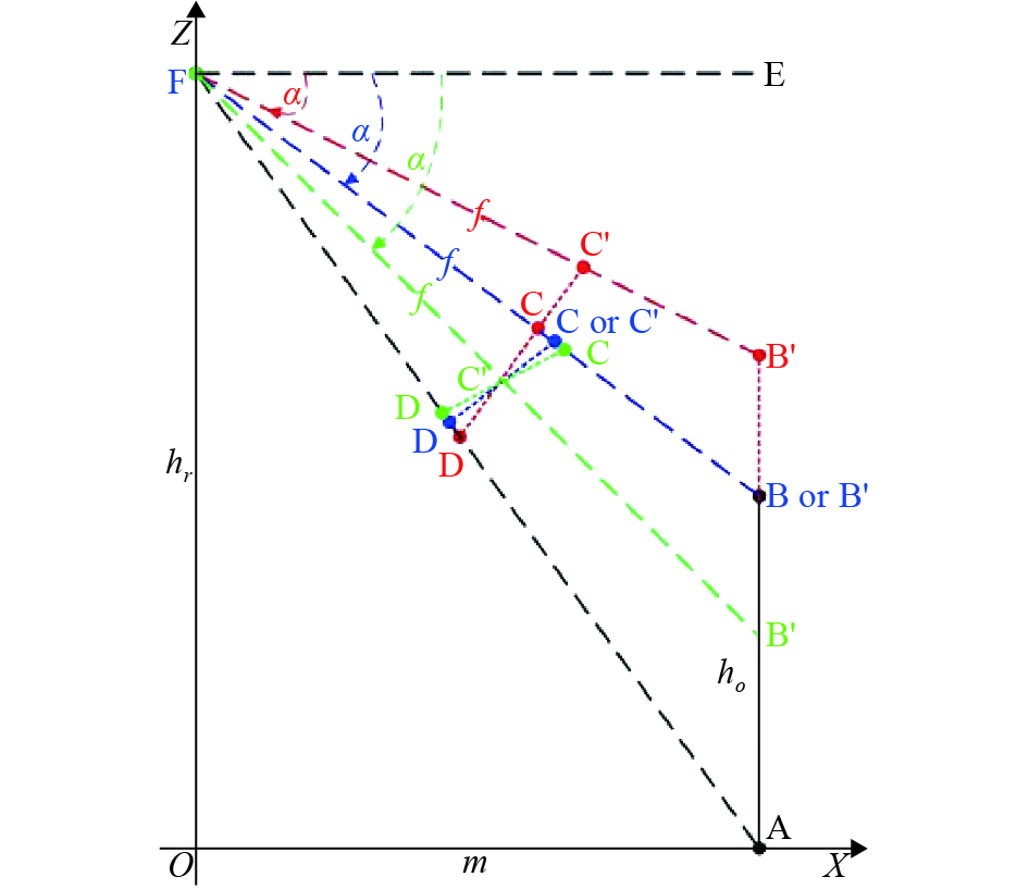
Figure 1. Two-dimensional geometric principle of camera imaging.
3.1. Model of camera imaging geometry with the target vertex falling on the main optical axis of the camera
When the highest point of the target just falls on the main optical axis of camera, it means that the target vertex is at the center of vision. To measure the horizontal distance between target AB and the camera, we use the bottom position of the camera as the center of the coordinate system, the horizontal line of the machine vision direction as X axis, and the line perpendicular to the OX axis on the ground plane as Y axis. Also, we set the camera position as point F, then the coordinate system shown in Figure 2 is established with the side of OF as Z axis. Suppose that the image plane is , the ground plane is , and the projected image plane is CD after the target AB is imaged by the camera. Obviously, points A, B, C, D, O and F are all on the plane where XOZ is located. Based on this, we can easily derive the relationship between the length , target distance , target height , and camera height :
From the basic principle of camera imaging, we know that since the vertex B of target |AB| falls on the main optical axis, the image C of point B must be the center of the image plane . Then, we can calculate the target distance as:
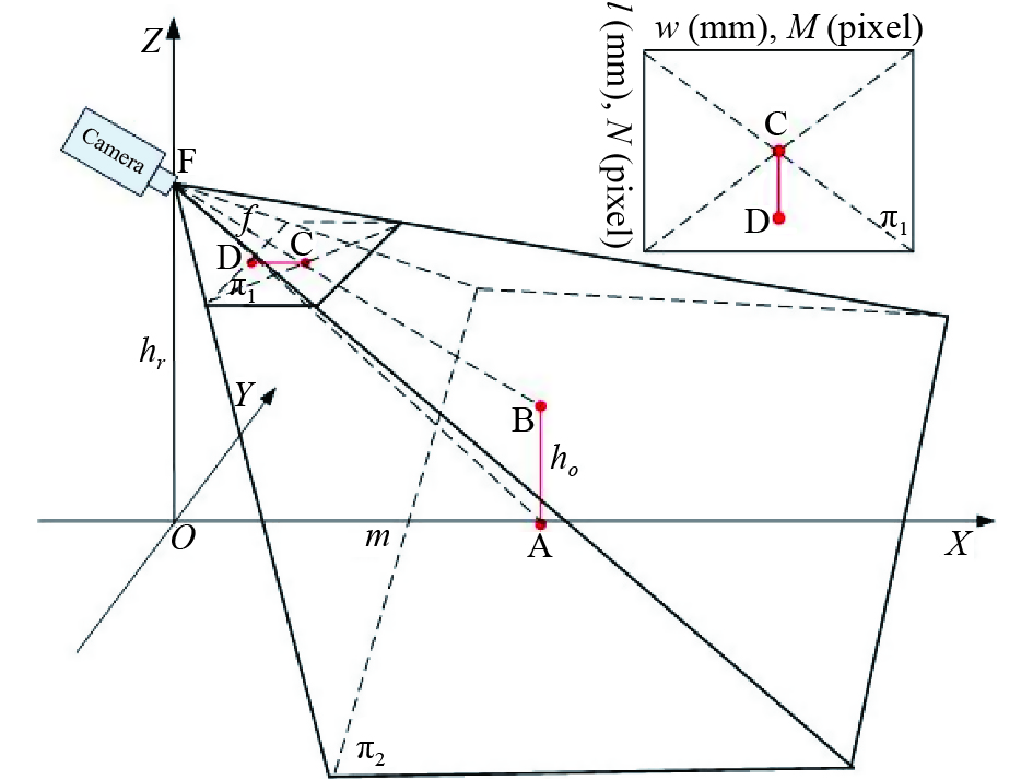
Figure 2. Schematic diagram of imaging with the target vertex falling on the main optical axis
3.2. Model of imaging geometry when the target vertex is higher than the main optical axis of the camera
When the target vertex is higher than the main optical axis of the camera, then in the image plane , the vertex C of the target image CD is higher than the center point of the image plane as shown in Figure 3. Suppose that the main optical axis of the camera and target AB intersect at point , and set , then . Consequently, we can easily obtain the following relationship of these parameters:
Finally, the relationship between the target height and the target distance can be written as:
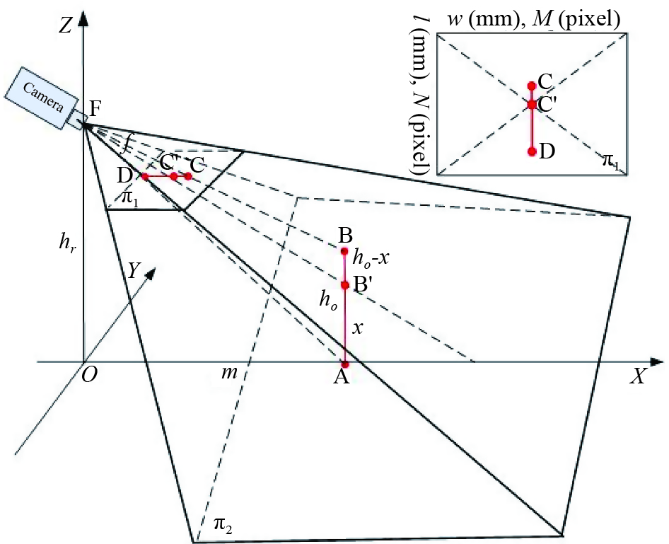
Figure 3. Schematic diagram of imaging when the target vertex is higher than the main optical axis of the camera.
3.3. Model of imaging geometry when the target vertex is lower than the main optical axis of the camera
When the target vertex is lower than the main optical axis of the camera, then in the image plane , the vertex C of the target image CD is lower than the center point of the image plane as shown in Figure 4. Suppose that the main optical axis of the camera and the extended line of target AB intersects at point , and set , then . Since the coordinates of CD in the image plane are and , and is the center point of the image plane, the simulation coordinates of are . We can express the target distance as:
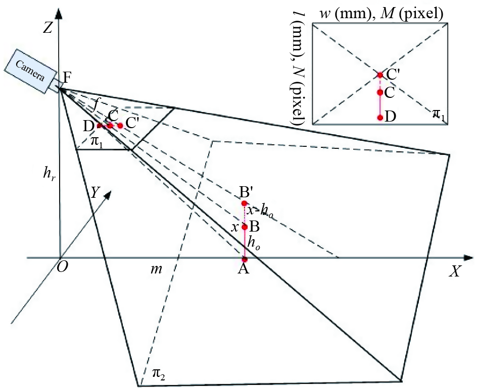
Figure 4. Schematic diagram of imaging when the target vertex is lower than the main optical axis of the camera.
3.4. Special model: relationship model of the target’s distance and height of the angle bisecting image
Definition 4:In a certain image acquisition process, if the main optical axis of the camera bisects the angle between two endpoints of the target and the camera. This kind of image is called the angle bisection image (ABI).
As shown in Figure 1, the main optical axis bisects , so we can easily derive the relationship between the depression angle and the CD length :
In Eq. (7), is the focal length of the camera, is the tangent function, , , and is the arctangent function.
Fig. 5 is a function diagram of the relationship between the depression angle and the target image length obtained with the target AB height 680 (mm), distance (mm), focal length of 50 (mm), and camera height of (mm). It can be seen from Figure 5 that when the depression angle gradually increases from zero, the CD length d gradually decreases until it reaches a certain value. After that, it gradually increases. In other words, has a minimum value. Taking the derivative of Eq. (7), we can easily know that when , reaches the minimum value. This is due to:
Therefore, when the main optical axis is the bisector of (the green part in Figure 1), reaches the minimum value. According to the angle bisector theorem in geometry, we can get the following equation:
Based on Eq. (9), we can obtain the relationship between the target’s distance and height of ABI as:
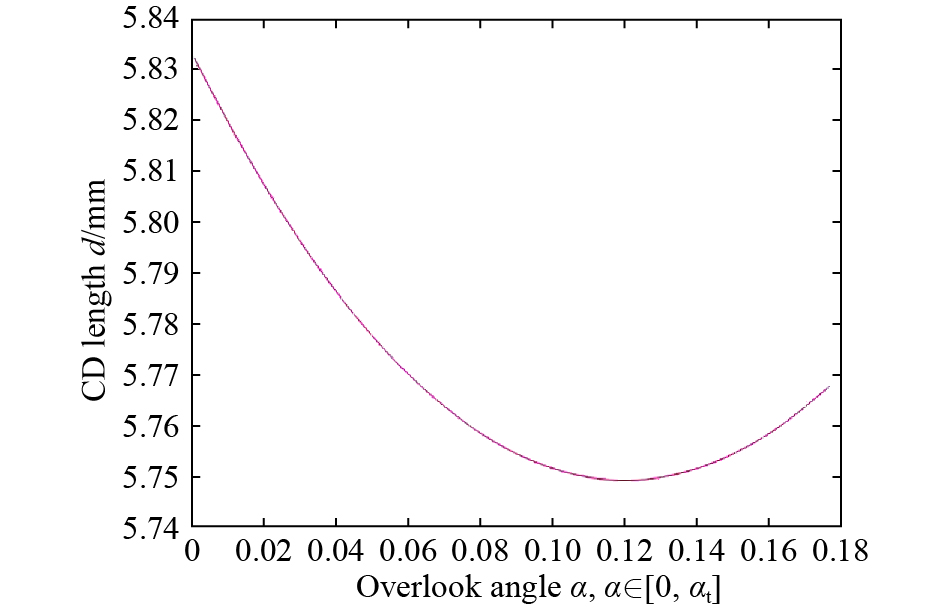
Figure 5. Relationship between the depression angle and target image CD length .
4. The solvability analysis of “self-invariance”
The “self-invariant” solvability analysis is to jointly solve above models without changing the camera’s height and the target’s distance to see whether the target distance and the target height can be solved. Before analyzing the solvability, we first agree on a joint solution symbol. The unknown variables for the joint solution of several equations are marked as “”. For example, means Eqs. (1) and (2) are used to perform the joint solution.
In Section 2, we derive four relational models. To discuss whether their joint form has a solution, we will first introduce a basic theory.
4.1. Infinite solutions of multi-model combination of a single frame image
The so-called single frame image multi-model combination refers to an image in which a single frame image satisfies two or more model conditions. For example, an ABI image does not only satisfy Eq. (10), but also satisfy Eqs. (5-1) and (5-2). To discuss whether there is a solution to the combination, we first introduce a basic theory.
4.1.1. Basic theory
For given camera parameters (including the camera height , focal length , photosensitive film size and image size ), can the target distance and target height be solved by single-frame image multi-model combination? In other words, does have a unique solution?
It seems that may have a unique solution. There are two unknown variables in Eq. (5), i.e., the target distance m, height , and the distance between the intersection of the main optical axis, the target and the lowest point of the target. Formula (5) has two equations (5-1) and (5-2), and Formula (10) has these three variables. With three equations and three variables, it seems that the target distance and height could be solved. However, has infinite solutions. In the following, we shall give a theorem about infinite solutions to joint multiple models of a single image.
Theorem 1: For any frame of the target image CD, under the condition of the same shooting height, images obtained from different depression angles will have different target heights and distances.
Proof: The equivalent meaning of the above theorem is that, given the height of target AB, the horizontal distance from the camera is and the obtained image is CD when the depression angle is . Under the condition that the camera height remains unchanged, change the depression angle and shoot. Let us set a new depression angle , that is, . Then, there must be a new target , so that the image of the new target is identical to the original target image CD, which is recorded as .To prove this theorem, we only need to prove its equivalence.
When shooting the target AB, the main optical axis is , the depression angle is , and the intersection of the main optical axis and image plane is . Obviously, is the center point of the image. Suppose the angle between the two endpoints of targets A and B and the camera is . That is, , which is shown by the black line in Figure 6.
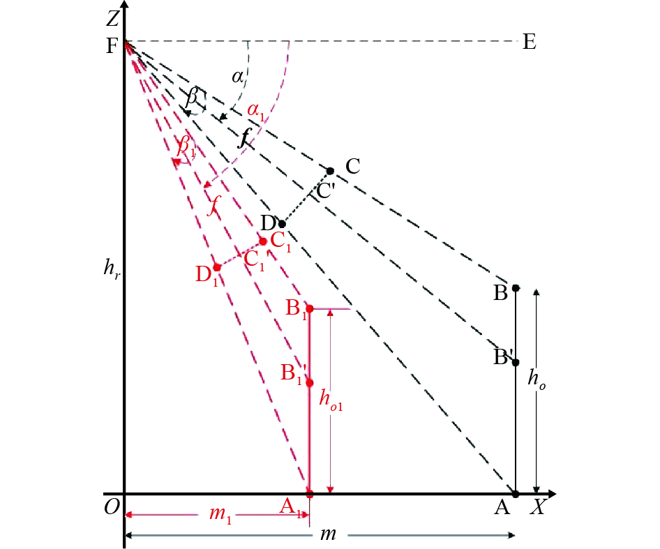
Figure 6. Principle of target imaging when rotating the main optical axis.
The conclusion of the above theorem is that , which means that the length of the target image does not change, and the position of the target image in the image does not change. This also means that the distance will not change between the two endpoints of the target image and the center point of the image plane . In the following section, we will employ a construction method to prove this conclusion.
The bind straight lines AF and BF to the active axis (that is, and ) remain unchanged, and can rotate around point F on the XOZ plane. When , the intersection points of the straight-line AF and the OX axis is , and a straight line parallel to AB is made through point , intersecting the main optical axis at and BF at respectively. This is shown in the red part in Figure 6. Since straight lines AF and BF are bound to , the image CD equivalent to AB is also bound to the AFB tripod. During rotation, , and always remain the same, i.e., , and are true. Also, since the focal length of the camera is fixed during the rotation, the length of the target image and the position information of the target image CD in the image will not change. Therefore, the target obtained is the new target, and the new target image is identical to the original target image CD. Therefore, is established. Proof completed.
According to Figure 6, we can clearly know that when , and hold. Of course, we can also see that the distance is a monotonically increasing function of the height . This theorem shows that the single-frame image multi-model combination cannot solve the two variables of the target distance and height . This is due to that a single frame image can only obtain the information of the target image CD, including the length of CD and the position information of CD in the image. We can only obtain the values of , and through this information. There are infinite number of targets satisfying this condition.
To further illustrate the conclusion of "the infinite solutions of the single-frame image multi-model joint", we take as an example and the details are described below.
4.1.2. infinite solution analysis
represents the problem of existence of the solution value of ABI. Therefore, the angle bisector image satisfies the condition that the main optical axis of the camera is lower than the target vertex and satisfies the angle bisector theorem in geometry.
In Eq. (11), is the distance from the center point of the image plane to point D of the image CD, and is the distance from the center point of image plane to point C of the image CD. Both and can be worked out by image segmentation and CD coordinates are obtained. Then, the digital transfer to the simulation method is shown in Figure 3. and represent the focal length and height of the camera, where represents the distance from the intersection point of the target and the optical axis to the ground, respectively, both of which are known beforehand. Therefore, there are only three unknown variables in the equation system, namely , , , and the equation system has three equations. From the number of equations and the number of variables, it seems that the equation can give the unique target height and target distance. Unfortunately, this equation also has an infinitely number of solutions.
The specific theoretical basis can be explained according to Theorem 1. We regard (11-1), (11-2), and (11-3) as three curved surfaces. In Figure 7, the subgraphs (a), (b) and (c) are three curved surfaces at the target height . It is a cross-sectional view of 580, 480, and 380. In each sub-graph, the three curves can intersect at one point. In other words, as the target height changes, a unique target distance value m can be obtained. The sub-figure (d) in Figure 7 is a cross-sectional view of . It can be seen from the sub-figure that the three curved surfaces intersect in a curve, not a point, and the target distance m increases monotonically along with the target height . This is consistent with our Theorem1.
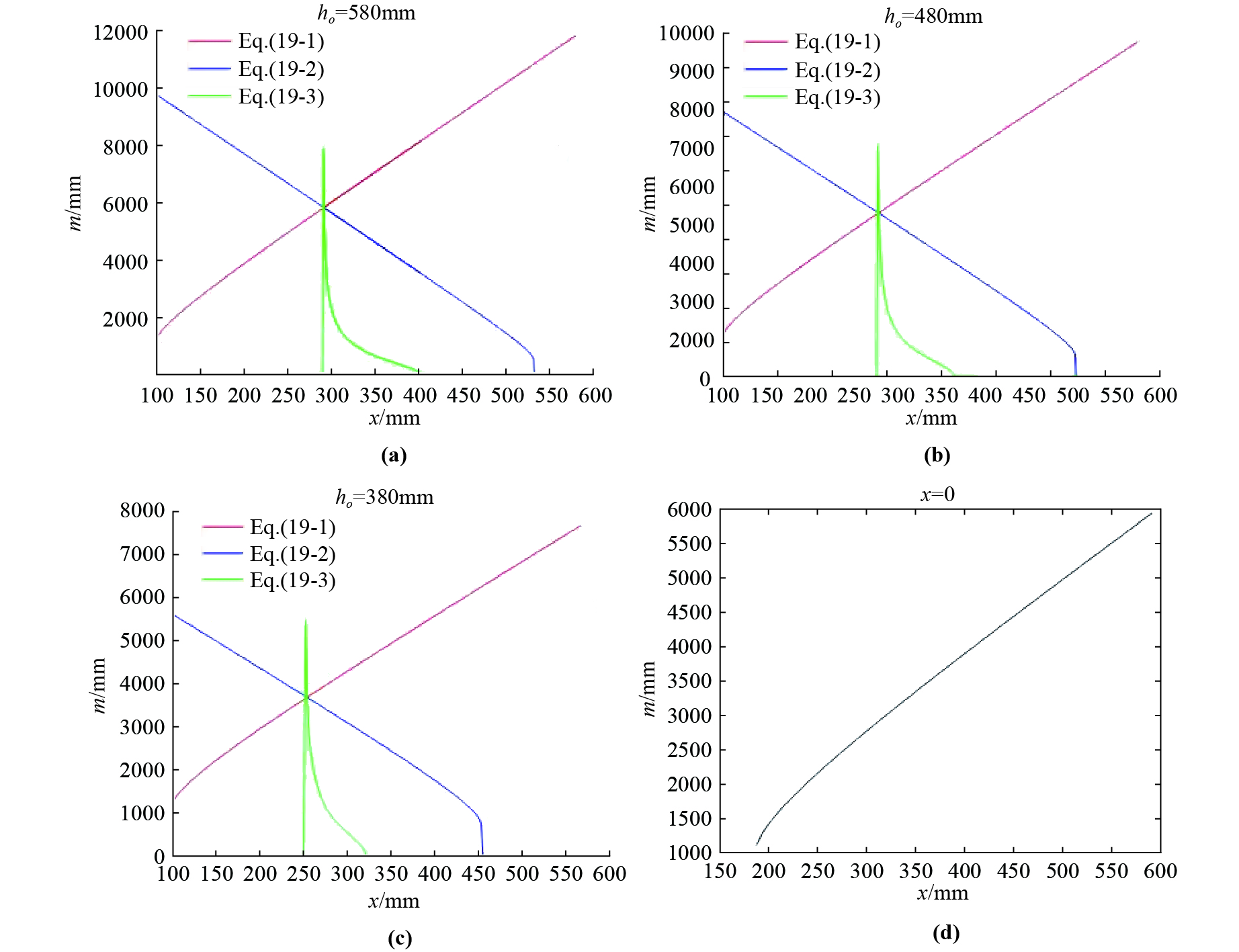
Figure 7. A sample diagram of with infinite solutions of the ABI image.
4.2. Infinite solutions of the multi-frame image joint
In Section 4.1, we have analyzed the infinite solutions of the single-frame image multi-model joint, that is, it is impossible to solve the target height and distance from a single frame image. So, can multiple images be used for the joint solution? For example, can we solve the target height and distance by combining different depression angle images? Let us first conduct theoretical analysis on this issue.
4.2.1. Basic theory
The multi-frame and multi-model joint situations with different depression angles are as follows. 1): represents a model when the target vertex happens to fall on the main optical axis and the target vertex is higher than the main optical axis. 2) represents a model when the target vertex happens to fall on the main optical axis and the target vertex is lower than the main optical axis. 3) represent a model when the target vertex is higher than the main optical axis and the target vertex is lower than the main optical axis. Since the ABI image is also a model with the target vertex higher than the main optical axis, we will not discuss the joint problem of the ABI image and other models.
and are three equations with three unknown variables , so the three unknown equations can be solved. In , there are four equations with four unknown variables , where is the distance from the lowest point of the target to the intersection point of the main optical axis of the camera and the target AB when the target vertex is higher than the main optical axis of the camera, and is the distance from the lowest point of the target to the intersection of the camera’s main optical axis and the target AB when the target vertex is lower than the camera's main optical axis. The four variables can also be solved. However, no matter for which set of equations, the unique target depth information cannot be found without knowing the target height. We first present a theorem as follows.
Theorem 2: Under the condition that the camera height the target height and the distance are unchanged, the target height obtained by the image taken at any depression angle is equivalent to the target distance relationship model.
Proof:
Suppose that shooting a target at a depression angle , the image obtained is , and the relationship model between the corresponding target height and distance is denoted as . When shooting a target at a depression angle , the image obtained is , and the relationship model between the corresponding target height and distance is denoted as . From a geometric point of view, on the plane , two curves (or straight lines) and appear. On the same plane, there are only three kinds of relationships between and : 1) and intersect but do not overlap. 2) and never intersect. 3) and coincide.
Under the condition that the target height and distance are unchanged, if we can prove that and coincide, then it is proved that the target height obtained by the image taken at any depression angle is equivalent to the target distance relationship model. Here, we use an elimination method to prove.
If we substitute into and respectively, and and are true, then it indicates that " and never intersect" will not hold. Below we use the method of proof by contradiction to prove that " and intersect but do not overlap" does not hold.
Assume that " and intersect but do not overlap" is true, that is, there is at least one point to make true but is invalid. Suppose that the target image corresponding to is . Based on Theorem 1, we know that holds. At this time, and hold. This contradicts our condition that “the target height and distance remain unchanged”. In other words, our hypothesis that “ and intersect but do not overlap” does not hold. Therefore, only one case that “ and coincide” holds. Proof completed.
It can be explained by Theorem 2 that the multi-frame image joint has infinite solutions. That is, the equations , , all have infinite solutions. In the following, we take as an example to further illustrate that has infinite solutions.
4.2.2. infinite solution analysis
Since Eq. (3) is a special form of Eq. (5) and (6), the infinite solutions of discussed is representative to a certain extent. Eq. (5) is the model of the imaging geometry when the target vertex is higher than the main optical axis of the camera. Eliminate the variable x in the Eq. (5) to obtain
Since , then
Eq. (6) is the model of the imaging geometry when the target vertex is lower than the main optical axis of the camera. Eliminate the variable in the equation (6) to obtain
Since , then
Since equations (13) and (15) are different models, the lengths of the target image in equations (13) and (15) are different, and the distances are also different from the lowest point and highest point of the target image to the center point of the image plane. To distinguish, we record the length of the target image, the distance from the lowest point of the target image to the center point of the image plane, and the distance from the highest point to the center point of the image plane in equation (15) as , and . Then, can be simplified to
When the height of the camera in Figure 8 is 1040mm and the focal length of the camera is 50mm, the image CD is obtained by shooting, and the coordinates (in pixel) are , , , . After calculating, we will get (in mm) , , , , and . In Figure 8, the two curves in the middle overlap completely. This further explains has infinite solutions.
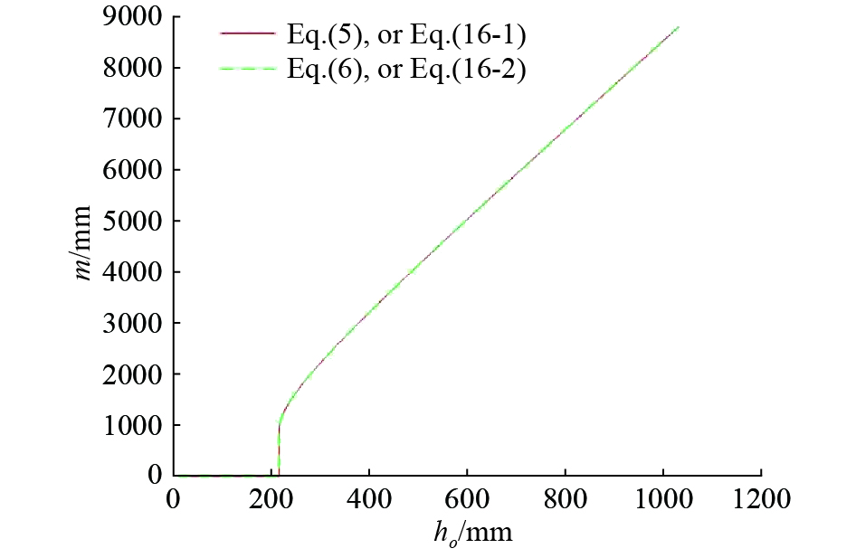
Figure 8. infinite solutions example graph.
5. Solvability analysis of “self-change”
From Section 1 we know that “self-change” is to change the two variable external parameters and . We will analyze the solvability of these two external parameters as follows.
5.1. Solvability analysis of changing the external parameter
In case a soft robot tracking the target, the external parameter can be changed during the machine learning process. The soft robot can change the external parameter by stretching its height. For example, the soft robot can stand on tiptoe or stretch its neck to observe the target. It can also bend down or shorten the neck to observe the target. In these cases, the external parameter will change. Suppose that the target image obtained by the robot at the height is , and the target image obtained after extending or shortening is , as shown in Figure 9. Then, the external parameter is
We stipulate as the positive direction, then when the robot is shortened, is negative, and when the robot is extended, is positive. Similarly, when the main optical axis is higher than the target vertex, is negative, When the main optical axis is lower than the target vertex, takes a positive value. In this way, we can substitute Eq. (17) into Eq. (16), and obtain joint solving equations with changing external parameters as follows:
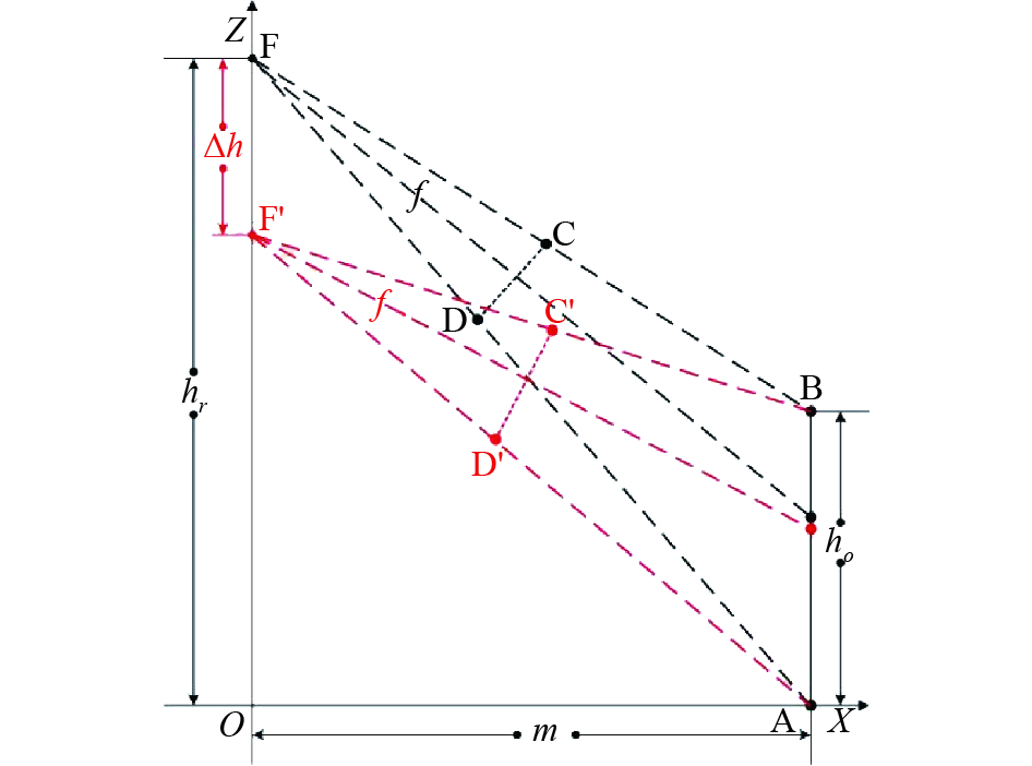
Figure 9. The imaging geometry principle of changing the external parameter .
,, in Eq. (18) represent the length of the target image in the image , the distance from to the image center, and the distance from to the image center, respectively, as shown in the red part in Figure 9. Then, we analyze whether there is a solution to the equation set (18). We denote the curve Eq. (18-1) as , and the curve Eq. (18-2) as . We take the partial derivative of on both sides of Eq. (18-1):
Since , Eq. (19) can be simplified to
The numerator part of Eq. (20) is . So, the denominator part determines the sign of the function . When , it is clear that is a monotonically increasing function with respect to , as shown in Figure 9. Since , the curvature of the curve is smaller than that of the curve . The intercept of the curve on the axis is , and the intercept of the curve on the axis of the axis is . This is due to , so That is, the intercept of the curve on the axis is smaller than the intercept of the curve on the axis, therefore, the curves of and have a unique intersection in the range. When , function and is monotonously decreasing, but the curvature of the curve is still smaller than the curvature of the curve . Since the intercept of the curve on the axis of the axis is smaller than the intercept of the curve ξ(I) on the axis, the curve ξ(I) and the curve have no intersection within the range of 0 < .
In summary, we can easily draw a simple graph of curves and , as shown in Figure 10. From Figure 10, we can see that there is only a unique intersection point between curves and in the range of , that is, there is a unique solution to the equation set (18).
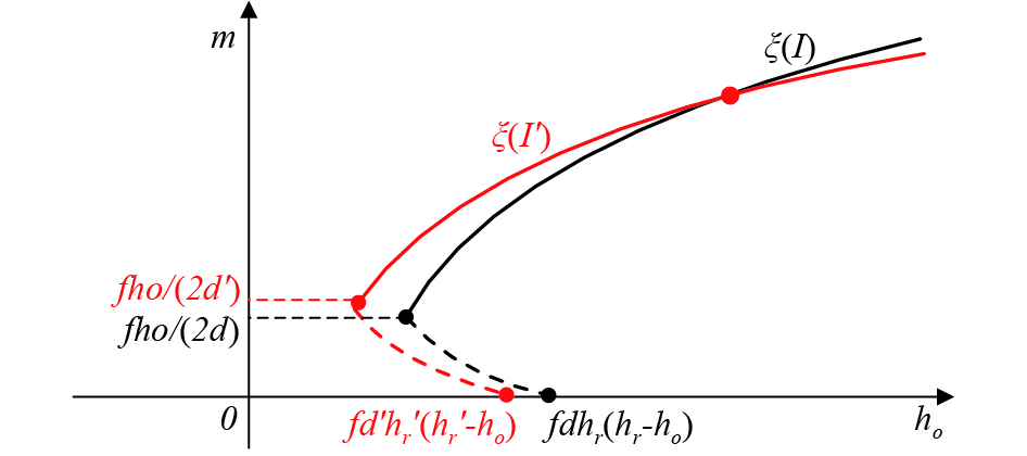
Figure 10. Approximate diagram of curves and when the external parameter changes.
5.2. Solvability analysis of changing external parameter
In case of a non-soft robot (e.g., a sliding robot and an unmanned car) tracking a target, it is difficult to learn the target’s height by changing its own height , but it is able to learn the target height by changing the external parameter . We can move forward or slide back to change the external parameter . Suppose that when the sliding robot is at height and the distance from the target is m, the target image obtained is , and the target image is obtained after sliding forward or backward by . As shown in Figure 11. the external parameter is
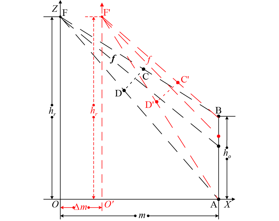
Figure 11. The imaging geometry principle of changing the external parameter .
We stipulate that is the positive direction. Then, when the robot approaches to the target, take the positive value, and when the robot moves backward, take the positive value of ∆m. In the target image, the direction is specified as the positive direction. Then, when equation (22) is substituted into equation (16), we have
, and in Eq. (22) represent the length of the target image in the image , the distance from to the image center, and the distance from to the image center, respectively, as shown in red in Figure 11.
Next, we analyze whether there is a solution to the equation set (22). Similarly, let us denote the curve formula (22-1) as and the curve Eq. (22-2) as , which are shown in Figure 12. We take the partial derivative of on both sides of equation (22-1):
When , the curvature of the curve increases monotonically. From Equation (23), it is difficult to judge the changing trend of the function with respect to the variable m. Therefore, we take the partial derivative of m with respect to the function as
When , 0, the curve is a monotonically increasing function with respect to , and the curvature of curve is larger than the curvature of curve . When ,, curve is a monotonically decreasing function with respect to , and the curvature of curve is smaller than the curvature of curve at this time. Therefore, is the turning point of curve , which are marked as the dark red dot in Figure 12.
Since the intercept of the curve on the axis changes from ) to , and when the observer approaches the target, the target distance decreases while the target image becomes larger, namely ,. Therefore, . The curve is at the upper left of the curve , as shown by the red dashed line in Figure 12. The red dashed line and the black curve will not intersect. It should be noted that in Figure 11 is a negative number since . Therefore, it is equivalent to shifting the curve to the right along the m axis to get the red solid curve in Figure 12. Although is greater than , . Therefore, the curves and will have two intersection points in the first quadrant, which are marked as blue points in Figure 12. That is, the solvability of the changing external parameter is true.
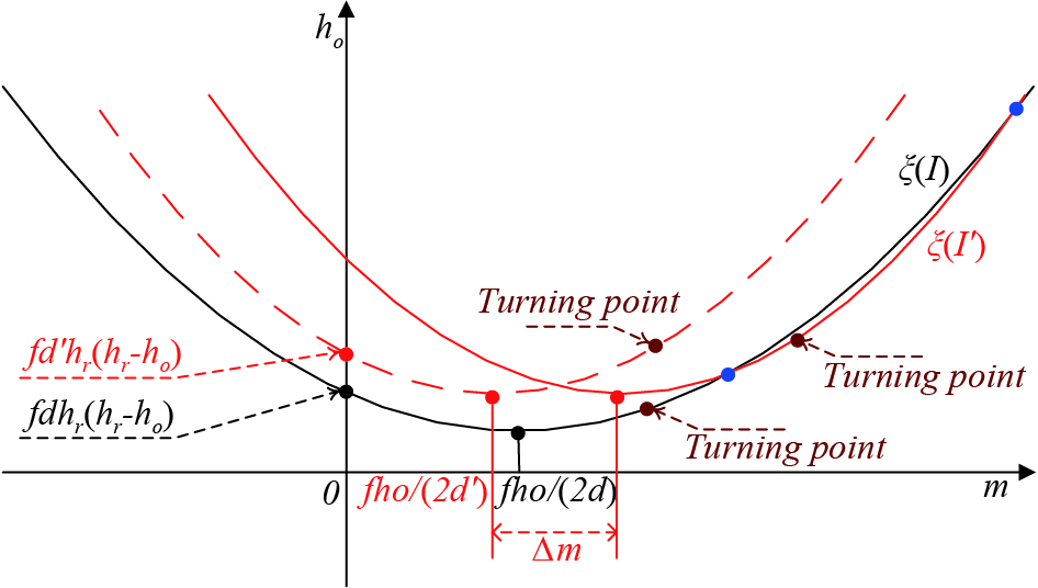
Figure 12. Approximate diagram of curves and when the external parameter changes.
6. Experimental Verification
To verify the correctness of our theory, we carried out the following experiments: 1) the target’s distance measurement experiment based on the change of the external parameter and 2) the target ’s height measurement based on the change of the external parameter .
6.1. Preparation
6.1.1. Experimental instrument
The experimental instrument is shown in Figure 13. The instrument is mainly composed of the camera and rangefinder. The rangefinder is used to measure the distance between the target and camera. The overhead control handle is used to control the depression angle when shooting. The rotator is used to adjust the direction of the camera so that the camera faces the target. The rotating console is used to control the horizontal rotation angle of the rotator, so that the lens can be aligned with the target. The variable-length bracket is used to control the height of the camera, and the telescopic range of the tripod bracket is 0.71-2.10 m.
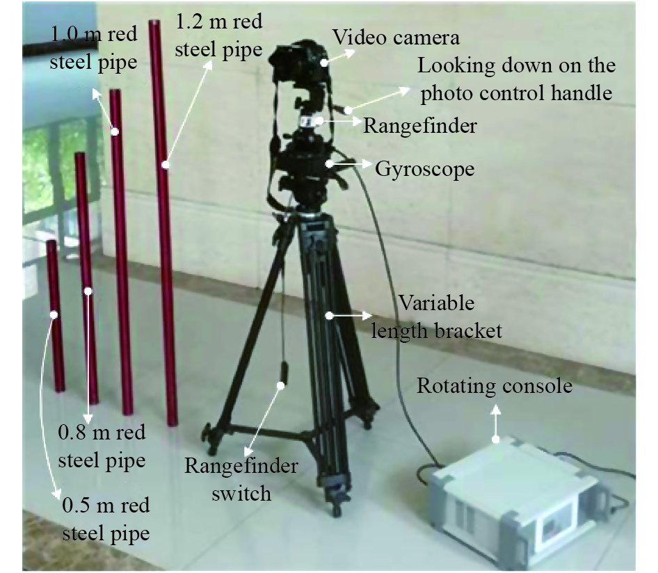
Figure 13. Experimental instrument.
To eliminate the error caused by the inaccurate target segmentation, we paint the target-strip steel pipe in red color. Such a target can be easily segmented by the color segmentation algorithm [40]. The lengths of the four target steel pipes are 120, 100, 80 and 50cm, respectively. The camera used in our experiment is SONY ILCE-7M2 with LAOWA Camera Lenses, which can reduce the error of target segmentation caused by distortion. The detailed parameters of the camera are shown in Table 1.
| Name | SONY ILCE-7M2 |
| sensor type | CMOS |
| Image size | 6000 × 4000(pixel) |
| Camera focal length f | 50(mm) |
| Aperture value | f/4 |
| 35 mm focal length | 50(mm) |
| Lens distortion type | Close-to-zero distortion |
6.1.2. Experimental data
We collect two sets of experimental data, and capture four steel pipes. Each has four camera heights and four different distances, a total of 16 sets of images. We take them as the target’s distance data based on the change of the external parameter (as shown in Table 2) and the target’s height data based on the change of the external parameter (as shown in Table 3). During the shooting process, we start shooting downwards from the axis slightly higher than the target vertex, so that each group of images has 5 cases: the main optical axis is higher than the target vertex, the main optical axis is slightly lower than the target vertex, the main optical axis falls near the midpoint of the target, the main optical axis is slightly higher than the lowest point of the target, and the main optical axis is lower than the lowest point of the target. These cases are labeled 1, 2, 3, 4, and 5 as shown in the first column in Figure 14.
| Target height (cm) | Target distance (cm) | Camera height (cm) | Amount |
| 50.0 | 160.0 | 148.5 | 5 |
| 165.0 | 5 | ||
| 240.0 | 110.0 | 5 | |
| 201.0 | 5 | ||
| 100.0 | 160.0 | 110.0 | 5 |
| 148.5 | 5 | ||
| 240.0 | 165.0 | 5 | |
| 201.0 | 5 |
| Target height(cm) | Camera height(cm) | Target distance(cm) | Amount |
| 80.0 | 110.0 | 240 | 5 |
| 320 | 5 | ||
| 165.0 | 160 | 5 | |
| 240 | 5 | ||
| 120.0 | 148.5 | 240 | 5 |
| 320 | 5 | ||
| 201.0 | 160 | 5 | |
| 240 | 5 |
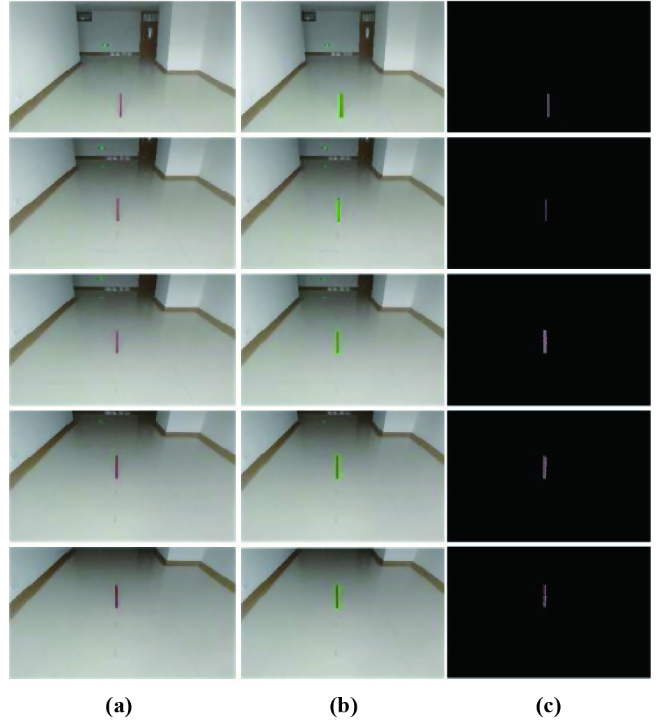
Figure 14. Sample image and target segmentation map.
6.2. Experimental results
To verify our theory and eliminate unnecessary errors caused by inaccurate segmentation, we manually segment the obtained images, which are shown in column (b) in Figure 14. The experimental results of these two kinds of the target’s height and distance are shown below.
6.2.1. Results of the target’s distance experiments based on the change of the external parameter
The meaning of the data in Table 2 is that the target height is and the distance between the target and camera is unknown. We need to learn the distance and the camera height is known. In this case, we first take a target image. Then, we change the height of the camera and take another target image. The camera change amount is , and this change amount is known beforehand. The height and distance of the target are obtained through the joint solution of the two images. We denote the target height and distance obtained by solving as .
We conducted experiments on the data in Table 2, and the experimental results are shown in Tables 4 and 5. Out of 50 trials with a target height of 50 cm (as shown in Table 4), the minimum error of the target height is 0.1 mm, and the maximum error is 11.6 mm. The minimum error of the target distance is 1.1324 mm, and the maximum error is 195.7346 mm. The average error of the target height is 2.54 mm, and the average error of the target distance is 33.414 mm.
| Image number j( |
||||||
| 1 | 2 | 3 | 4 | 5 | ||
| Image number i ( | 1 | (500.1,1605.8) | (500.5,1616.2) | (500.1,1607.8) | (499.6,1594.3) | (499.6,1594.9) |
| 2 | (500.2,1607.6) | (500.6,1618.0) | (500.3,1609.5) | (499.7,1596.0) | (499.9,1598.9) | |
| 3 | (500.1,1605.9) | (500.5,1616.3) | (500.2,1607.8) | (499.6,1594.4) | (499.6,1595.0) | |
| 4 | (500.2,1607.6) | (500.6,1618.0) | (500.3,1609.5) | (499.7,1560.0) | (499.8,1602.6) | |
| 5 | (500.2,1607.8) | (500.6,1618.2) | (500.3,1609.7) | (499.8,1596.2) | (499.8,1596.8) | |
| Image number j() | ||||||
| 1 | 2 | 3 | 4 | 5 | ||
| Image number i ( | 1 | (498.7,2398.6) | (488.8,2207.2) | (498.6,2397.2) | (497.0,2367.7) | (497.6,2379.3) |
| 2 | (498.2,2395.2) | (488.4,2204.3) | (498.1,2293.7) | (496.5,2364.3) | (497.1,2379.9) | |
| 3 | (498.1,2384.8) | (488.3,2203.9) | (498.1,2393.3) | (507.2,2542.0) | (497.1,2375.5) | |
| 4 | (499.1,2400.9) | (498.1,2209.1) | (499.0,2399.4) | (508.2,2548.9) | (498.0,2381.5) | |
| 5 | (500.1,2407.6) | (500.9,2420.7) | (500.1,2406.2) | (498.3,2376.5) | (499.0,2388.2) | |
| Image number j() | ||||||
| 1 | 2 | 3 | 4 | 5 | ||
| Image number i( | 1 | (1005.9,1628.8) | (1000.2,1605.5) | (1000.1,1605.0) | (999.9,1604.0) | (1001.2,1609.6) |
| 2 | (999.2,1605.0) | (999.8,1604.5 | (999.7,1604.0) | (999.5,1603.0) | (1000.8,1608.6) | |
| 3 | (1001.3,1608.4) | (1001.2,1607.9) | (1001.1,1607.5) | (1000.8,1606.4) | (1002.2,1612.1) | |
| 4 | (1002.9,1612.4) | (1002.8,1611.9) | (1002.4,1610.4) | (1002.4,1610.4) | (1003.8,1616.0) | |
| 5 | (999.9,1604.8) | (999.8,1604.3) | (999.6,1603.9) | (999.4,1602.8) | (1000.8,1608.5) | |
| Image number j() | ||||||
| 1 | 2 | 3 | 4 | 5 | ||
| Image number i ( | 1 | (999.8,2403.1) | (998.5,2394.4) | (1000.9,2405.9) | (998.5,2394.5) | (1001.7,2414.6) |
| 2 | (1000.9,2407.5) | (999.5,2398.8) | (1001.9,2414.3) | (999.5,2398.9) | (1002.7,2419.0) | |
| 3 | (1000.0,2404.0) | (1001.1,2410.7) | (998.7,2395.4) | (998.7,2395.4) | (1001.9,2415.5) | |
| 4 | (997.6,2393.4) | (996.2,2384.8) | (998.7,2400.1) | (996.3,2384.8) | (999.4,2404.8) | |
| 5 | (1002.4,2414.4) | (1001.0,2405.7) | (1003.5,2421.2) | (1001.1,2405.7) | (1004.3,2426.0) | |
Out of 50 trials with a target’s height of 100 cm (as shown in Table 5), the minimum error of the target’s height is 0.1 mm, the maximum error is 5.9 mm, the minimum error of the target distance is 0.1 mm, and the maximum error is 28.8 mm. The average error of the target height is 2.076 mm, and the average error rate of the target distance is 8.792 mm.
From the results of the changing external parameter (Table 4 and Table 5), the target height and distance calculated by our method are awfully close to their true values, and there is a proportional relationship between the target height and distance error. The group of the large target height error also shows a large target distance error. Conversely, if the target height error is small, the target distance error is also small. These experimental data illustrate the feasibility of our target’s distance method.
6.2.2. Results of the target’s height experiment based on the change of the external parameter
The meaning of the data in Table 3 is that the target height is and the distance between the target and camera m is unknown. We need to learn the distance, and the camera height is known beforehand. In this case, we take a target image. Then, we move closer to the target or stay away from the target, that is, we change the distance and shoot the target again to obtain another target image. The target distance is changed with a value of , and this value is known beforehand. The height and distance of the target are obtained through the joint solution of the two images. In this experiment, we take the larger number as our original distance. For example, given m= (mm) and m= (mm), we take m=3200 mm, then (mm). Therefore, the value of calculated by our experiment is the distance before the initial target change.
We conduct experiments on the data in Table 3, and the experimental results are shown in Tables 6 and 7. In the experiment with a target height of 80 cm, the minimum error of the target height is 0.003 mm, the maximum error is 11.1 mm, and the average error is 2.442 mm. The minimum error of the distance is 0.3 mm, the maximum error is 52.5 mm, and the average error is 13.886 mm.
| Image number j() | ||||||
| 1 | 2 | 3 | 4 | 5 | ||
| Image number i ( | 1 | (803.6,3223.6) | (791.9,3169.5) | (803.6,3223.5) | (796.3,3189.6) | (800.2,3207.8) |
| 2 | (811.1,3252.5) | (798.8,3196.1) | (810.5,3250.1) | (803.2,3216.2) | (807.7,3236.5) | |
| 3 | (807.9,3240.3) | (795.7,3183.9) | (807.3,3237.9) | (800.0,3204.0) | (804.5,3224.4) | |
| 4 | (799.7,3208.6) | (796.2,3186.1) | (799.7,3208.4) | (792.4,3174.6) | (796.3,3192.7) | |
| 5 | (802.0,3217.5) | (800.7,3203.4) | (802.0,3217.3) | (795.1,3185.2) | (798.6,3201.5) | |
| Image number j() | ||||||
| 1 | 2 | 3 | 4 | 5 | ||
| Image number i ( | 1 | (799.5,2398.2) | (800.1,2401.1) | (800.2,2401.6) | (799.6,2398.5) | (799.9,2400.3) |
| 2 | (801.5,2415.8) | (802.1,2419.5) | (802.2,2420.1) | (801.7,2416.8) | (801.9,2418.7) | |
| 3 | (799.3,2395.7) | (799.9,2399.2) | (800.0,2399.8) | (799.4,2396.7) | (799.7,2398.5) | |
| 4 | (799.4,2396.8) | (800.0,2400.3) | (800.1,2400.9) | (799.5,2397.8) | (799.9,2396.6) | |
| 5 | (799.8,2400.7) | (801.3,2412.0) | (801.4,2412.6) | (800.8,2409.4) | (801.1,2411.3) | |
| Image number j() | ||||||
| 1 | 2 | 3 | 4 | 5 | ||
| Image number i ( | 1 | (1217.8,3261.0) | (1200.7,3203.4) | (1209.3,3232.5) | (1206.7,3223.6) | (1214.1,3248.4) |
| 2 | (1213.1,3247.2) | (1196.0,3189.1) | (1204.6,3218.4) | (1202.0,3209.5) | (1209.4,3234.5) | |
| 3 | (1217.8,3260.9) | (1200.7,3203.3) | (1209.3,3232.4) | (1206.7,3223.5) | (1214.1,3248.3) | |
| 4 | (1210.5,3239.2) | (1193.2,3180.9) | (1201.9,3210.4) | (1199.2,3201.4) | (1206.7,3226.6) | |
| 5 | (1216.6,3257.5) | (1197.7,3193.7) | (1208.2,3229.0) | (1205.5,3220.0) | (1212.9,3245.0) | |
| Image number j() | ||||||
| 1 | 2 | 3 | 4 | 5 | ||
| Image number i ( | 1 | (1198.3,2392.5) | (1198.2,2391.6) | (1199.7,2398.8) | (1199.6,2395.8) | (1198.4,2392.6) |
| 2 | (1199.4,2402.2) | (1199.2,2401.3) | (1200.7,2408.7) | (1200.4,2408.3) | (1199.4,2402.4) | |
| 3 | (1199.1,2399.5) | (1198.9,2398.7) | (1200.4,2406.0) | (1200.4,2405.6) | (1199.1,2399.7) | |
| 4 | (1218.0,2516.1) | (1217.6,2514.7) | (1220.4,2526.8) | (1220.3,2526.2) | (1198.6,2395.1) | |
| 5 | (1199.7,2405.4) | (1199.5,2404.5) | (1201.1,2411.9) | (1201.0,2411.6) | (1199.7,2406.8) | |
In the experiment with a target height of 120 cm, the minimum error of the target height is 0.3 mm, the maximum error is 30.4 mm, and the average error is 5.916 mm. The minimum error of the distance is 1.2 mm, the maximum error is 126.8 mm, and the average error is 25.9 mm.
The above target’s height experiment results (Table 6 and Table 7) reveal that the target information (the height and distance) calculated by our method has a small deviation from the true values. Further, there is a proportional relationship between the target height deviation and the target distance deviation. If the height deviation is large, the distance deviation is also large. The closer the target height is to the actual height, the closer the distance is to the actual distance. This indeed shows the correctness of our target’s height theory of changing the external parameter .
It should be noted that from Table 4 to Table 7, it is difficult to see whether the errors have a certain relationship or, whether this combination has higher (lower) accuracy. To ascertain this, further statistical analysis is required as shown below.
6.2.3. Analysis of experimental results
In the measurement field, the measurement error is often a direct reflection of measurement accuracy [40]. In order to analyze measurement accuracy, two methods of combining stability analysis and measurement stability analysis in the uncertainty theory are often used for experimental analysis.
Combination stability analysis is use to examine the advantages and disadvantages of various combinations. This method is to verify whether changes in the camera’s tilt angle during the shooting process has an impact on the measurement results. For example, although the first and second shots meet the “self-change” conditions, there may be errors in the measurement results when the second shot has a different upward or downward viewing angle and the second shot has the same upward or downward viewing angle.
Measurement stability analysis is used to analyze the stability of our measurement method, that is, to check whether the measurement data obtained from each measurement is stable. The purpose of this paper is to detect whether the measurement effect is better when the targets in two images are far apart or when the distance is closer.
6.2.3.1. Combination stability analysis
To compare the performance of various combinations, we have calculated the average error rate of each combination. For example, the combination, which means the joint solution of two images when the main optical axis is higher than the target vertex and the main optical axis is slightly lower than the target. The calculation method of the average error rate of the joint solution is
In Eq. (25), and represent the target height and distance, respectively, obtained by , and represent the quantity of the combination of . For example, in means the number of combinations of in Table 4 to Table 7. Since the joint solution of two images satisfies the commutability, that is, , it is obvious that holds.
The average error results are shown in Table 8. The best combination is while the combination shows the worst performance. It should be noted that it is difficult for us to conclude types of images with better effects and types of images with worse effects. Therefore, we have further calculated the marginal error rate statistics.
| Joint | Er(·)(%) | Joint | Er(·)(%) | Joint | Er(·)(%) | ||
| 0.5194 | 0.7549 | 0.6266 | |||||
| 0.6316 | 0.6266 | 0.5756 | |||||
| 0.3178 | 0.7776 | 1.3171 | |||||
| 0.6535 | 0.4406 | 0.4514 | |||||
| 0.2951 | 0.3938 | 0.5148 | |||||
| (%) | |||||||
| 0.5050 | 0.6463 | 0.5083 | 0.7652 | 0.5037 | |||
| (%) | |||||||
| 0.1532 | 0.1120 | 0.1278 | 0.2950 | 0.1058 |
Definition 5: The marginal error rate refers to the average of each type of image error, denoted as: . The calculation method of is shown in Eq. (26):
The calculation results of are shown in Table 8. In terms of marginal error rate, the experimental results of 1, 3, and 5 types of images are relatively close, and the performance of 2, 4 types of images are relatively inferior. Which one is the most stable type of image? To answer this question, we calculated the standard deviation of the marginal error rate (denoted as ), as is shown in the last row in Table 8. Based on the standard deviation, we find images of categories 2, 3, and 5 are relatively stable, while images of category 4 are unstable.
Although our experimental results are relatively good, the calculated results have a certain deviation from the true values. After carefully studying the reasons for deviations, we believe that these deviations are mainly caused by target segmentation, target imaging distortion and the accuracy of our measuring instruments.
6.2.3.2. Measurement stability analysis
In order to analyze the stability of our measurement algorithm, that is, to check whether the measurement data obtained in each measurement is stable, we use the uncertainty measure method [40] to analyze the stability of our measurement method. The calculation method of uncertainty measure is defined as:
where denotes the uncertainty measure of the target height, represents the uncertainty measure of the target distance, is the standard deviation of the unbiased estimate, is the number of measurements, is the sample measurement value, is the mean value, and is the error of instrument which is generally calculated by half of the minimum division of the instrument [41]. Since we measure the true value of the target height and distance, the committed step is the segmentation of the target in the image. The minimum division of image segmentation is one pixel. From Section 6.1, we can see that the size of CMOS is =(mm) and the size of the image is (pixel). The focal length f of the camera is 50 mm, and is used to approximate the straight-line distance between the target and camera lens. Then,
According to the above equation, the error of the camera itself is proportional to the target distance and inversely proportional to the resolution of the camera. Since two images are needed for each measurement and the target distance is different when the image is taken, we take the average value of the instrument error when the two images are taken as the instrument error . Eq. (27) is used to calculate Tables 4 to 7, respectively, and the results are shown in Table 9. In Table 9, “Up” represents the statistical results for the upper part of Tables 4 to 7, while “Down” represents the statistical results for the lower part of Tables 4 to 7. The uncertainty measure of the target height is less than the uncertainty measure of the target distance. However, from the experimental results (Tables 2 and 3), the target distance is greater than the target height. From the results, we can see that the smaller value of the measured target will lead to better stability.
| Table 4 | Up | 0.3641 | 12.1738 | 0.1155 |
| Down | 4.5031 | 87.9528 | 0.1593 | |
| Table 5 | Up | 1.6207 | 5.5001 | 0.1201 |
| Down | 2.0730 | 10.7510 | 0.1777 | |
| Table 6 | Up | 5.2454 | 22.6999 | 0.1690 |
| Down | 0.9521 | 8.3896 | 0.1307 | |
| Table 7 | Up | 6.8509 | 22.6125 | 0.1689 |
| Down | 7.3627 | 44.9677 | 0.1322 | |
The value of the uncertainty measure is far greater than the value of the instrument error, so the measurement stability of our method is high. However, our measurement accuracy depends on the accuracy of target segmentation and distortion of the camera. We therefore further analyze the segmentation accuracy and camera distortion and discuss the impact of these issues on the target height and distance measurement.
6.3. Discussion
The experimental results in Section 6.2 show the correctness of our theory. In real applications, errors between the target information are calculated by our method and the actual value exists. These errors mainly come from target segmentation and camera distortion. We should discuss and analyze these two issues below.
6.3.1. The impact of segmentation accuracy on target’s height and distance
To verify our theory and reduce the error of target’s height and distance caused by imprecise target segmentation, we paint the steel pipe red. Therefore, we use the red target segmentation method for target segmentation [39, 42], and the specific method is shown by formula (26).
In Eq. (29), , , represent the gray value of the RGB color component of the image I, and , and represents the threshold value of the difference between the R color component and the G and B color components. Through training and learning, , are set to be 20 and 22, respectively. Column (c) in Figure 14 is the target image of column (a) obtained by the segmentation of the algorithm.
We conduct experiments on the data in the first column of Table 2 and Table 3. Table 10 shows the results of manual segmentation and the target segmentation obtained by color segmentation. There is a certain error between manual segmentation and color segmentation. The maximum error differs by 8 pixels, and the minimum error differs by 2 pixels. The average correlation between the two is 4.5 pixels.
We employ the proposed method to calculate the target height and distance based on color segmentation, and the results are shown in Table 10. Compared with the calculation results of manual segmentation, the error of color segmentation is obviously much larger.
| , | |||||||||
| Image number | |||||||||
| Manual segmentation | Color segmentation | Manual segmentation | Color segmentation | ||||||
| 1 | 2825 | 3760 | 2828 | 3759 | 2871 | 3717 | 2876 | 3715 | |
| 2 | 1844 | 2699 | 1850 | 2697 | 1799 | 2571 | 1797 | 2572 | |
| 3 | 1470 | 2320 | 1472 | 2318 | 1586 | 2355 | 1590 | 2354 | |
| 4 | 1154 | 2010 | 1148 | 2011 | 1183 | 1957 | 1188 | 1956 | |
| 5 | 393 | 1296 | 388 | 1297 | 579 | 1384 | 575 | 1384 | |
| , | |||||||||
| Image number | |||||||||
| Manual segmentation | Color segmentation | Manual segmentation | Color segmentation | ||||||
| 1 | 2399 | 3831 | 2400 | 3830 | 2650 | 3772 | 2652 | 3771 | |
| 2 | 1868 | 3195 | 1870 | 3192 | 1844 | 2886 | 1845 | 2885 | |
| 3 | 1294 | 2620 | 1295 | 2618 | 1584 | 2617 | 1585 | 2616 | |
| 4 | 689 | 2038 | 695 | 2040 | 1135 | 2170 | 1138 | 2170 | |
| 5 | 171 | 1576 | 174 | 1575 | 326 | 1417 | 330 | 1417 | |
To test the impact of target segmentation accuracy on target’s height and distance, we assume that our manual segmentation is accurate. We use Equation (29) to calculate the target height deviation per pixel (denoted as: ) and target distance deviation per pixel (denoted as: ):
In Eq. (28), , is the manual segmentation target length of the i-th image, and is the color segmentation target length of the i-th image. We use Eq. (28) to calculate the experimental results of the change of the external parameter (the upper part of Table 11) and the change of the external parameter m (the lower part of Table 11). pixel). and of the external parameter are (mm/pixel) and (mm/pixel) and and of the external parameter m are (mm/pixel) and (mm/pixel). From the experimental results, when changing the external parameter , the pixel deviation is more sensitive to the target distance, but not sensitive to the target height. Every time a pixel is changed, the target height may have about 2mm deviation. Changing is more sensitive to the target height, but not to the target distance. Every time a pixel deviation occurs, the target distance will change by 8 mm, and the average values are (mm/pixel) and (mm/pixel). Overall, for each deviation of 1 pixel, the target height deviation is about 2.5 mm, and the height deviates by about 1.5 cm. Therefore, the impact of target segmentation on target’s height and distance is small.
| , | ||||||
| Image number j() | ||||||
| 1 | 2 | 3 | 4 | 5 | ||
| Image number i ( | 1 | (493.1,1498.7) | (493.3,1508.2) | (493.1,1500.5) | (492.8,1488.2) | (492.9,1488.7) |
| 2 | (504.4,1662.4) | (504.9,1673.3) | (504.5,1664.4) | (503.8,1650.3) | (503.8,1650.9) | |
| 3 | (494.5,1523.0) | (494.8,1532.7) | (494.6,1524.8) | (494.3,1512.2) | (494.3,1512.8) | |
| 4 | (491,2,1464.1) | (491.4,1473.4) | (491.2,1465.9) | (491.1,1453.9) | (491.1,1454.4) | |
| 5 | (517.6,1811.9) | (518.4,1824.3) | (517.7,1814.2) | (516.7,1798.1) | (516.7,1798.8) | |
| , | ||||||
| Image number j() | ||||||
| 1 | 2 | 3 | 4 | 5 | ||
| Image number i ( | 1 | (789.7,3209.9) | (787.6,3152.4) | (789.6,3161.6) | (788.4,3155.9) | (798.5,3202.9) |
| 2 | (793.0,3175.0) | (790.9,3165.3) | (792.9,3174.5) | (791.7,3168.8) | (801.9,3215.9) | |
| 3 | (793.0,3174.9) | (790.9,3165.2) | (792.9,3174.4) | (791.7,3168.7) | (801.8,3215.8) | |
| 4 | (788.3,3156.7) | (786.2,3147.0) | (788.2,3156.2) | (786.9,3150.4) | (797.1,3197.5) | |
| 5 | (785.8,3147.0) | (783.7,3137.3) | (785.7,3146.5) | (784.5,3140.7) | (794.6,3187.8) | |
6.3.2. The impact of camera distortion on target’s height and distance
To test the impact of camera distortion on target’s height and distance, we use the NIKON D7100 camera as the data collecting camera. NIKON D7100 is a SLR camera launched by Nikon in 2013 (the camera focal length f is 50mm, the sensor size is 23.5 × 15.6 mm, and the image size is 6000 × 4000 pixel). The conversion relationship between the focal length of this camera and the 135-size camera is 1.5 magnification.
We collect two sets of data with this camera. In the first one, the target height is 50 cm, the camera height is 191.5 cm or 147 cm, and the target distance is 400 cm. In the second group, the target height is 50 cm, the camera height is 179 cm, and the target distance is 320 cm or 400 cm. The shooting starts from the situation where the main optical axis is higher than the target vertex to the main optical axis and lower than the lowest point of the target. 10 images are taken in each group, which are used to test the impact on target’s height and distance when the external parameter and the external parameter change. We use the color segmentation algorithm for target segmentation, and the experimental results are shown in Figure 15 and Figure 16.
It can be seen from Figure 15 and Figure 16 that the deviation between the calculated and true target height and distance is exceptionally large. We have calculated the average error of the target height and distance, which are 55.6624 mm and 490.3100 mm, respectively. It can be concluded that the distortion of the camera has a great impact on target’s height and distance.
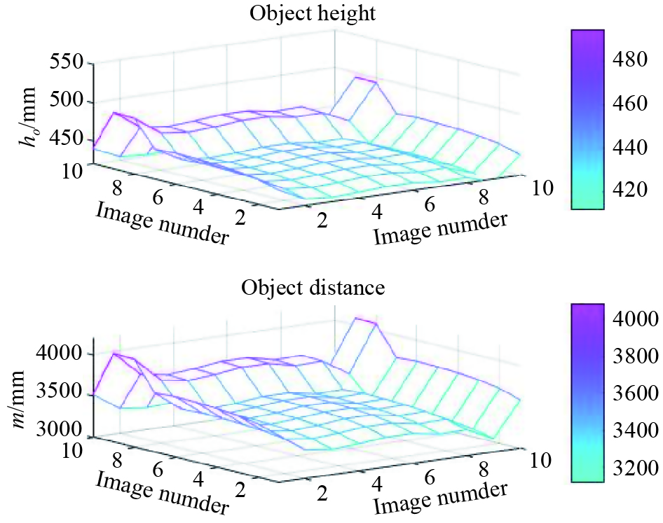
Figure 15. The target’s distance result of the NIKON D7100 camera with changing external parameter .
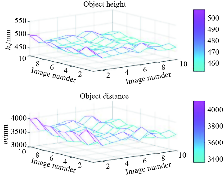
Figure 16. The target’s height result of the NIKON D7100 camera with changing external parameter .
We also correct the camera distortion. The correction method calculates in advance the incident angle of the target vertex and the lowest point of the target to the camera. For example, in the set of experiments where the target height is 50 cm, the target distance is 400 cm, and the camera height is 191.5 cm, we obtain that the incident angle of the target vertex α_1 is , and the incident angle of the lowest point of the target α_2 is 0.4465. Then, the distortion factor is:
In Eq. (31), , and are the focal length of the camera, the distance from the lowest point of the target image to the image center, and the distance from the highest point of the target image to the image center, respectively. Correct and by :
In Eq. (32), and are the correction values of and , respectively. We conduct experiments on the first group based on above formula, and the experimental results are shown in Figure 17.
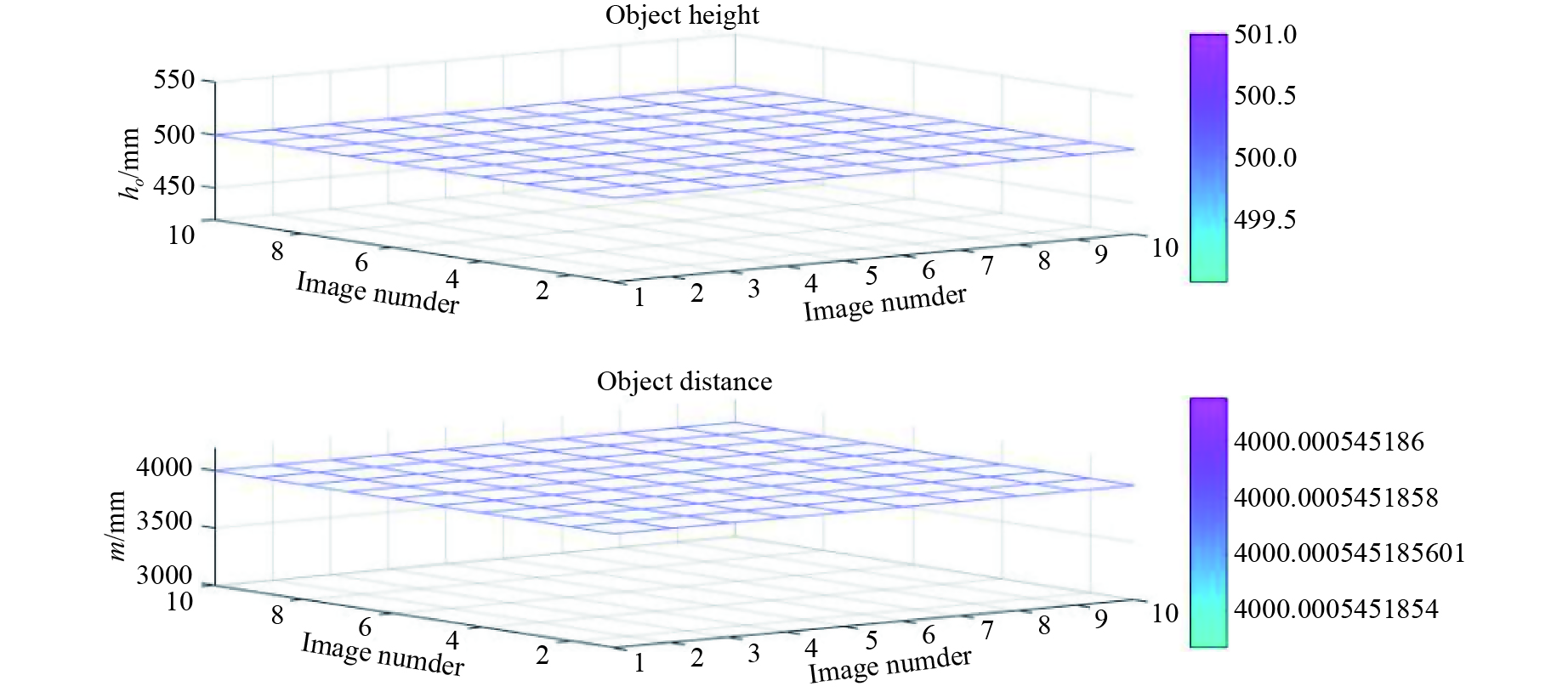
Figure 17. Camera distortion correction results from Figure 15.
It can be seen from Figure 17 that through distortion correction, the accuracy is extremely high, the average error of the target height is mm, the average error of the distance is mm, and the precision reaches the nanometer level. It can be seen from Equation (29) that through this correction, the target segmentation error has been corrected.
This correction method is not applicable in real engineering, as it is impossible for us to calculate the incident angle between the target vertex and the lowest point of the target in advance. However, this set of experiments does show the correctness of our theory.
6.3.3. Comparison with previous works
Early target depth information learning methods mainly focus on binocular camera perception methods that mimic human eyes, target depth information estimation methods based on deep learning, and monocular cameras + other equipment depth acquisition methods.
Jia et al. [10] developed an omni-directional 3D camera system consisting of the camera, hyperbolic mirror, infrared laser diodes and diffractive of element (DOE), to obtain the 3D depth information. Francisco [13] calculated depth information from two cameras arranged in a stereoscopic manner by using continuous changes in the distance between the lens plane and the image plane (primary distance). Yang et al. [14] proposed a 3D hand tracking method using a binocular stereo camera to obtain key depth information of the target to understand the characters that the user writes in the air. Mao et al. [19] proposed the single camera plus the flat mirror method to measure the target depth in the water. This method can only be performed in a close-up environment and is not suitable for moving robots to track the target. Xu et al. [21] propose a depth model which fuses complementary information derived from multiple CNN side outputs. Different from previous methods using concatenation or weighted average schemes, the integration is obtained by means of continuous Conditional Random Fields (CRFs). Eigen et al. [27] proposed a method to solve the depth prediction problem by using two deep network stacks. This helps achieve depth prediction through rough global prediction and local refinement of this prediction.
Tateno et al. [31] proposed a dense depth map predicted by the CNN to naturally merge the depth measurement values obtained from direct monocular SLAM. This fusion scheme prioritizes depth prediction at image locations where the monocular SLAM method tends to fail. David et al. [32] used a single basic architecture to solve the deep prediction problem. They used a multi-scale convolutional network to directly regress from the input image to the output map. Our method uses a series of scales to gradually refine the prediction and capture many image details without any super pixels or low-level segmentation. Mao et al. [35] proposed the single camera plus the flat mirror method to measure the target depth in the water. This method can only be performed in a close-up environment and is not suitable for moving robots to track the target. Tong Jia et al. [43] proposed a depth sensing system based on the monochromatic shape encoding decoding structured light method, which is designed to scan the surface of an object and sense its depth. The system includes a commercial projector and a monochrome CCD camera. Using DenseNet for depth detection of scanned object surfaces, the attempted detection accuracy is as high as 96%.
Dongxue Li et al. [44] proposed a multi-state object depth acquisition method based on binocular structured light, which utilizes two cameras and a projector to obtain depth information of static and moving targets. The authors proposed a scene depth perception method based on omnidirectional structured light with a depth error of 0.04mm for static targets.
Jia Tong et al. [45] utilized a projector, a hyperbolic mirror, and a camera to avoid the influence of occlusion and achieve an average measurement error of 0.25cm by using the 3D reconstruction technology. The accuracy of the depth measurement in these literatures is significantly better than the methods proposed in this article (with an average measurement error of 0.6595%). However, the equipment of these methods is significantly more complex than that of this article, and these three technologies are mainly applicable to the reconstruction of 3D targets in specific scenes. Although accurate depth information is obtained, such methods are difficult to be applied to the measurement of the target height and depth in outdoor situations.
We conduct qualitative and quantitative experimental comparisons using methods in literature [10, 13, 14, 19, 21, 27, 31, 35, 43, 44, 45] and our method. The comparison results are shown in Table 12. From Table 12, it can be seen that the method proposed in this article has the best stability, with an average error of only 0.5857%. The literature [14] has the worst stability, with an average depth estimation error of 3.7865%. Compared with these methods, our method has three advantages: 1) it can be used to accurately calculate the depth and height of the target; 2) it is simple, with low computational complexity, and is easy to be implemented; 3) it can be used for both target tracking and target measurement.
The “Pinhole camera model”, which has been widely used in computer vision field, could describe the vision measurement problem clearly and succinctly. By comparison, the advantages of our proposed algorithm are three-fold. Firstly, the measurement instrument is simplified. In our method, only one camera is required, i.e., other auxiliary equipment, such as another camera, hyperbolic mirror, and infrared laser diodes, is not necessary. Secondly, the algorithm is simplified. We use geometry to obtain two sets of equations, which has lower complexity compared to computationally intensive neural networks. Finally, the amount of data to be processed is small. In our method, only the data from a single camera needs to be processed. Compared to the data in those algorithms which require other auxiliary equipment, the data to be proposed in our algorithm is rather small.
| Works | Methods | Target | Results | Average Error |
| [10] | One Camera, hyperbolic mirror, infrared laser diodes | Indoor target | Target depth | 0.6300% |
| [13] | Two Cameras | Ground target | relative depth map | 2.4623% |
| [14] | Two Cameras | hand tracking | character recognition | 3.7865% |
| [19] | One Camera, Multiple CNN | Ground target | Depth Estimation | 0.8967% |
| [21] | A multi-scale deep network | A singe image | Depth map prediction | 1.8754% |
| [27] | Monocular SLAM, CNNs | A singe image | Depth measurements | 0.9563% |
| [31] | A multiscale convolutional network | A singe image | Depth prediction | 5.6830% |
| [35] | One Camera, a mirror | fish | Underwater target depth | 0.9758% |
| [43] | One Camera, one projector | Scanning objects | deep inspection | 0.6468% |
| [44] | Two Cameras, one projector | Static and moving targets | depth inspection | 0.7002% |
| [45] | A hyperbolic mirror, one camera, one projector | Scanning objects | depth inspection | 0.5986% |
| ours | One camera | Ground target | Target depth and height | 0.5857% |
6.3.4. Engineering applicability analysis - measurement method of target distance non-vertical to the ground
The algorithm in this paper theoretically solves the problem of using monocular parallax to obtain the target height and target distance. In theory, the target is required to be vertical to the ground. However, in certain practical engineering applications, such as automatic obstacle avoidance of autonomous vehicles, only the distance of the obstacle needs to be measured, while the height of the obstacle is irrelevant. Therefore, we only need to detect the prominent point of obstacles on the vertical centerline of the image, segment the pixel from the ground at that point, and finally calculate the target distance.
To verify this theory, we simulate an automatic obstacle avoidance scenario of an autonomous vehicle. Suppose that there is an obstacle (i.e., a parked e-bike) on the road, which is not vertical to the ground. The e-bike will be observed for the first time (shown in the first column in Figure 18) and when the autonomous vehicle moves forward, the same e-bike will be observed (shown in the second column in Figure 18). Since the edge of the e-bike’s pedal is white, which is regarded as a prominent part of the obstacle. The highest part of the e-bike corresponding to the vertical centerline of the image is the seat cushion, which is regarded as a key part. Connect the two wheels of the e-bike with the ground contact point and intersect the centerline of the image at point A, which is the lowest point of the obstacle. Then, the centerline of the image crossing the highest point of the white pedal edge of the e-bike can be regarded as the prominent point of the prominent part and recorded as . Connecting , which is the target vertical to the ground, as shown in the red segment in the first row of Figure 18, we mark the highest point of the e-bike crossing the centerline of image as . Connect , which is also regarded as a target vertical to the ground, as shown in the green segment in the second row in Figure 18.
How to automatically segment a prominent point of the target in image and the distance of this point to the ground pixel is not a concern of this paper. So, the segmentation is carried out manually to complete the above operation. We collect two different distance target images with the camera height of 1084mm and target distances of 8390mm, 7615mm and 4980mm, respectively. The resulting images are marked as , such as represents the image taken when the target distance is 8390mm, and the target is the e-bike’s pedal.
We denote the test result as , for example, represents the calculated result of the target distance between and . We employ the proposed method to calculate . The obtained results are that , , , , and . The average error of the target distance among the six sets of test data is 208.6mm, which means the relative error rate is about 2.5%. Since the autonomous vehicle is equipped with a taximeter, the distance traveled by the vehicle can be calculated. Based on this information, our proposed algorithm can be employed to calculate the distance between the target and autonomous vehicle in real time, thus realizing automatic obstacle avoidance. Therefore, the algorithm proposed in this paper can be applied to certain real applications.
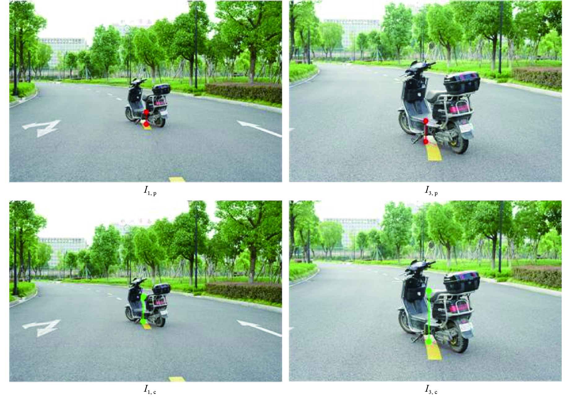
Figure 18. Obstacle target which is not vertical to the ground (e-bike). In and , the pedals are regarded as the prominent points with 8390mm and 4980mm, respectively. While in and , the key points are the seat cushions with 8390mm and 4980mm, respectively.
7. Conclusions
Target information measurement is one of the key technologies in computer vision. Extensive research has been carried out on this subject. This paper has proposed a target’s height and distance measurement method based on monocular vision. According to the principle of camera imaging and basic principles of analog-to-digital conversion, we theoretically prove the insolvability of “self-invariance” and the solvability of “self-change”. Based on the theory, the relationship has been analyzed between the target distance, target height, camera focal length, camera height and image resolution can be deduced, and the monocular target’s measurement. The experimental results have shown that the theory proposed in this paper is correct, and the algorithm is simple and easy to be implemented, which can effectively reduce the cost of production. Due to the simple structure of the monocular depth measurement system, it can be widely used in mobile phones and web cameras to avoid the complicated stereo matching process of the distance measurement by binocular cameras and reduce computational complexity.
Author Contributions: Mao Jiafa is the corresponding author and is primarily responsible for writing the manuscript, coding experimental programs, and revising the manuscript. Zhang Lu is mainly responsible for proofreading the English grammar and collecting experimental data.
Funding: National Natural Science Foundation of China (No. 62176237), The “Pioneer” and “Leading Goose” R&D Program of Zhejiang Province (Grant No. 2023C01022).
Data Availability Statement: If readers need experimental data, they can request it from the corresponding author Mao Jiafa.
Conflicts of Interest: We declare that we have no financial and personal relationships with other people or organizations that can inappropriately influence our work, there is no professional or other personal interest of any nature or kind in any product, service and/or company that could be construed as influencing the position presented in, or the review of, the manuscript entitled, “Basic theories and methods of target’s height and distance measurement based on monocular vision”.

References
- Qian, D.W.; Rahman, S.; Forbes, J.R. Relative constrained SLAM for robot navigation. In
2019 American Control Conference (ACC), Philadelphia, PA, United States, 10 –12 July 2019 ; IEEE: New York, 2019; pp. 31–36. doi: 10.23919/ACC.2019.8814592 - Lv, W.J.; Kang, Y.; Zhao, Y.B. FVC: A novel nonmagnetic compass. IEEE Trans. Ind. Electron., 2019, 66: 7810−7820. doi: 10.1109/TIE.2018.2884231
- Hachmon, G.; Mamet, N.; Sasson, S.; et al. A non-Newtonian fluid robot. Artif. Life, 2016, 22: 1−22. doi: 10.1162/ARTL_a_00194
- Tan, K.H. Squirrel-cage induction generator system using wavelet petri fuzzy neural network control for wind power applications. IEEE Trans. Power Electron., 2016, 31: 5242−5254. doi: 10.1109/TPEL.2015.2480407
- Kong, L.F.; Wu, P.L.; Li, X.S. Object depth estimation using translations of hand-eye system with uncalibrated camera. Comput. Integr. Manuf. Syst., 2009, 15: 1633−1638,1663. doi: 10.13196/j.cims.2009.08.179.konglf.027
- Hoang, N.B.; Kang, H.J. Neural network-based adaptive tracking control of mobile robots in the presence of wheel slip and external disturbance force. Neurocomputing, 2016, 188: 12−22. doi: 10.1016/j.neucom.2015.02.101
- Mendes, N.; Neto, P. Indirect adaptive fuzzy control for industrial robots: A solution for contact applications. Expert Syst. Appl., 2015, 42: 8929−8935. doi: 10.1016/j.eswa.2015.07.047
- Ghommam, J.; Mehrjerdi, H.; Saad, M. Robust formation control without velocity measurement of the leader robot. Control Eng. Pract., 2013, 21: 1143−1156. doi: 10.1016/j.conengprac.2013.04.004
- Charalampous, K.; Kostavelis, I.; Gasteratos, A. Thorough robot navigation based on SVM local planning. Robot. Auton. Syst., 2015, 70: 166−180. doi: 10.1016/j.robot.2015.02.010
- Jia, T.; Shi, Y.; Zhou, Z. X.; et al. 3D depth information extraction with omni-directional camera. Inf. Process. Lett., 2015, 115: 285−291. doi: 10.1016/j.ipl.2014.09.029
- Shirmohammadi, S.; Ferrero, A. Camera as the instrument: The rising trend of vision based measurement. IEEE Instrum. Meas. Mag., 2014, 17: 41−47. doi: 10.1109/MIM.2014.6825388
- Lee, C.R.; Yoon, K.J. Confidence analysis of feature points for visual-inertial odometry of urban vehicles. IET Intell. Transp. Syst., 2019, 13: 1130−1138. doi: 10.1049/iet-its.2018.5196
- Francisco, A. Continuous principal distance change for binocular depth perception. Image Vis. Comput., 1995, 13: 101−109. doi: 10.1016/0262-8856(95)93151-H
- Yang, J.C.; Xu, R.; Ding, Z. Y.; et al. 3D character recognition using binocular camera for medical assist. Neurocomputing, 2017, 220: 17−22. doi: 10.1016/j.neucom.2016.01.122
- Xu, Y.; Guo, D.X.; Zheng, T.X.;
et al . Research on camera calibration methods of the machine vision. In2th International Conference on Mechanic Automation and Control Engineering, Hohhot, 15–17 July 2011 ; IEEE: New York, 2011; pp. 5150–5153. doi: 10.1109/MACE.2011.5988241 - Li, J.; Allinson, N.M. A comprehensive review of current local features for computer vision. Neurocomputing, 2008, 71: 1771−1787. doi: 10.1016/j.neucom.2007.11.032
- Song, L.M.; Wu, W.F.; Guo, J.R.;
et al . Survey on camera calibration technique. InProceedings of Fifth International Conference on Intelligent Human-Machine Systems and Cybernetics, Hangzhou, China, 26 –27 August 2013 ; IEEE: New York, 2013; pp. 389–392. doi: 10.1109/IHMSC.2013.240 - Sun, J.; Gu, H.B. Research of linear camera calibration based on planar pattern. World Acad. Sci. Eng. Technol., 2011, 60: 627−631.
- Abdel-Aziz, Y.I.; Karara, H.M. Direct linear transformation into object space coordinates in close-range photogrammetry. In
Proceedings Symposium on Close Range Photogrammetry, Urbana, Illinois, 1971 ; 1971; pp. 1–18. - Tsai, R. A versatile camera calibration technique for high-accuracy 3D machine vision metrology using off-the-shelf TV cameras and lenses. IEEE J. Robot. Autom., 1987, 3: 323−344. doi: 10.1109/JRA.1987.1087109
- Zhang, Z.Y. Camera calibration with one-dimensional objects. IEEE Trans. Pattern Anal. Mach. Intell., 2004, 26: 892−899. doi: 10.1109/TPAMI.2004.21
- Zheng, F.; Tang, H.B.; Liu, Y.H. Odometry-vision-based ground vehicle motion estimation with SE(2)-constrained SE(3) poses. IEEE Trans. Cybern., 2019, 49: 2652−2663. doi: 10.1109/TCYB.2018.2831900
- Xu, D.; Ricci, E.; Ouyang, W.L.; et al. Monocular depth estimation using multi-scale continuous CRFs as sequential deep networks. IEEE Trans. Pattern Anal. Mach. Intell., 2019, 41: 1426−1440. doi: 10.1109/TPAMI.2018.2839602
- Liu, F.Y.; Shen, C.H.; Lin, G.S.; et al. Learning depth from single monocular images using deep convolutional neural fields. IEEE Trans. Pattern Anal. Mach. Intell., 2016, 38: 2024−2039. doi: 10.1109/TPAMI.2015.2505283
- Eigen, D.; Puhrsch, C.; Fergus, R. Depth map prediction from a single image using a multi-scale deep network. In
Proceeding of the 27th International Conference on Neural Information Processing Systems, Montreal, Canada, 8 –13 December 2014 ; MIT Press: Cambridge, 2014; pp. 2366–2374. - He, L.; Wang, G.H.; Hu, Z.Y. Learning depth from single images with deep neural network embedding focal length. IEEE Trans. Image Process., 2018, 27: 4676−4689. doi: 10.1109/TIP.2018.2832296
- Zhang, Z.Y.; Xu, C.Y.; Yang, J.; et al. Deep hierarchical guidance and regularization learning for end-to-end depth estimation. Pattern Recognit., 2018, 83: 430−442. doi: 10.1016/j.patcog.2018.05.016
- Loo, S.Y.; Amiri, A.J.; Mashohor, S.;
et al . CNN-SVO: Improving the mapping in semi-direct visual odometry using single-image depth prediction. InInternational Conference on Robotics and Automation (ICRA), Montreal, QC, Canada, 20 –24 May 2019 ; IEEE: New York, 2019; pp. 5218–5223. doi: 10.1109/ICRA.2019.8794425 - Tateno, K.; Tombari, F.; Laina, I.;
et al . CNN-SLAM: Real-time dense monocular slam with learned depth prediction. In2017 IEEE Conference on Computer Vision and Pattern Recognition (CVPR), Honolulu, HI, United States, 21 –26 July 2017 ; IEEE: New York, 2017; pp. 6565–6574. doi: 10.1109/CVPR.2017.695 - Eigen, D.; Fergus, R. Predicting depth, surface normals and semantic labels with a common multi-scale convolutional architecture. In
IEEE International Conference on Computer Vision, Santiago, Chile, 7 –13 December 2015 ; IEEE: New York, 2015; pp. 2650–2658. doi: 10.1109/ICCV.2015.304 - Wang, P.; Shen, X.H.; Lin, Z.;
et al . Towards unified depth and semantic prediction from a single image. In2015 IEEE Conference on Computer Vision and Pattern Recognition (CVPR), Boston, MA, United States, 7 –12 June 2015 ; IEEE: New York, 2015; pp. 2800–2809. doi: 10.1109/CVPR.2015.7298897 - Li, B.; Shen, C.H.; Dai, Y.C.;
et al . Depth and surface normal estimation from monocular images using regression on deep features and hierarchical CRFs. In2015 IEEE Conference on Computer Vision and Pattern Recognition (CVPR), Boston, MA, United States, 7 –12 June 2015 ; IEEE: New York, 2015; pp. 1119–1127. doi: 10.1109/CVPR.2015.7298715 - Cao, Y.Z.H.; Wu, Z.F.; Shen, C.H. Estimating depth from monocular images as classification using deep fully convolutional residual networks. IEEE Trans. Circuits Syst. Video Technol., 2018, 28: 3174−3182. doi: 10.1109/TCSVT.2017.2740321
- Zheng, K.C.; Zha, Z.J.; Cao, Y.;
et al . LA-Net: Layout-aware dense network for monocular depth estimation. In26th ACM Multimedia Conference, Seoul, Korea, 22 –26 October 2018 ; ACM: New York, 2018; pp. 1381–1388. doi: 10.1145/3240508.3240628 - Mao, J.F.; Xiao, G.; Sheng, W.G.; et al. Research on realizing the 3D occlusion tracking location method of fish’s school target. Neurocomputing, 2016, 214: 61−79. doi: 10.1016/j.neucom.2016.05.067
- Hemelrijk, C.K.; Hildenbrandt, H.; Reinders, J.; et al. Emergence of oblong school shape: Models and empirical data of fish. Ethology, 2010, 116: 1099−1112. doi: 10.1111/j.1439-0310.2010.01818.x
- Yao, J.L.; Yan, H.M.; Zhang, X.D.; et al. Image registration and superposition for improving ranging accuracy of imaging laser radar. Chin. J. Lasers, 2010, 37: 1613−1617. doi: 10.3788/CJL20103706.1613
- Cai, H.; Hu, Z.Z.; Huang, G.; et al. Integration of GPS, monocular vision, and high definition (HD) map for accurate vehicle localization. Sensors, 2018, 18: 3270. doi: 10.3390/s18103270
- Mao, J.F.; Huang, W.; Sheng, W.G. Target distance Measurement method using monocular vision. IET Image Process., 2020, 14: 3181−3187. doi: 10.1049/iet-ipr.2019.1293
- Liu, B.D.
Uncertainty Theory , 4th ed.; Springer: Berlin, Heidelberg, 2015; pp. 9–26. doi: 10.1007/978-3-662-44354-5 - Qin, Z.F. Developments of conditional uncertain measure. In
8th International Conference on Information and Management Sciences, Kunming, China, 20–28 July 2009 ;2009 ; pp. 802–806. - Wang, X.F. The Study of Level Set Methods and Their Applications in Image Segmentation. Ph.D. Thesis, University of Science and Technology of China, Hefei, China,
2009 . (In Chinese). - Jia, T.; Yuan, X.; Gao, T.H.Q.; et al. Depth perception based on monochromatic shape encode-decode structured light method. Opt. Lasers Eng., 2020, 134: 106259. doi: 10.1016/j.optlaseng.2020.106259
- Li, D.X.; Jia, T.; Wu, C.D.; et al. Multi-state objects depth acquisition based on binocular structured light. Opt. Lasers Eng., 2019, 121: 521−528. doi: 10.1016/j.optlaseng.2019.05.003
- Jia, T.; Wang, B.N.; Zhou, Z.X.; et al. Scene depth perception based on omnidirectional structured light. IEEE Trans. Image Process., 2016, 25: 4369−4378. doi: 10.1109/TIP.2016.2590304