Downloads
 Download


This work is licensed under a Creative Commons Attribution 4.0 International License.
Article
Multi-Dimensional Adaptive Learning Rate Gradient Descent Optimization Algorithm for Network Training in Magneto-Optical Defect Detection
Yiping Liang, Lulu Tian *, Xu Zhang, Xiao Zhang, and Libing Bai
School of Automation Engineering, University of Electronic Science and Technology of China, Sichuan 611731, China
* Correspondence: lulutian@uestc.edu.cn
Received: 24 September 2023
Accepted: 8 November 2023
Published: 25 September 2024
Abstract: As an optimization technique, the gradient descent method is widely adopted in the training process of deep learning. In traditional gradient descent methods, the gradient of each dimension has the same weight wtih the updating direction, which results in poor performances when there are multiple small gradient dimensions (e.g. near the saddle point). To improve the accuracy and convergence speed of the neural network training, we propose a novel multi-dimensional adaptive learning rate gradient descent optimization algorithm (M-AdaGrad) in this paper. Specifically, in the M-AdaGrad, the learning rate will be updated according to a newly designed weight function related to the current gradient. Experiments on a set of sigmoid-based functions verify that, compared with traditional gradient descent methods such as AdaGrad and Adam, the M-AdaGrad gives more confidence to the larger gradient direction and has a larger probability to reach a more optimal position with a faster speed. Due to its excellent performance in network training, the M-AdaGrad is successfully applied to the magneto-optical nondestructive test of crack detection based on the generative adversarial network.
Keywords:
multi dimension adapted learning rate gradient descent optimization neural network nondestructive test crack detection1. Introduction
In the past decade, the deep learning neural networks have developed rapidly and attracted much attention in a large number of applications including image processing [1–4] and speech recognition [5–7]. Different novel structures of neural networks have been proposed to analyse big and high dimension data, such as the convolutional neural networks (CNN) [8–10], generative adversarial networks (GAN) [11–13], auto-encoder [14–16], long-short term memory (LSTM) [17, 18] and graph neural networks (GNN) [19–21]. Usually, a neural network model is designed to solve a specific complex problem such as feature extraction, information classification, data generation and data prediction. For these complex tasks, the nonlinear activation functions (e.g. the sigmoid function and 'relu' function) are commonly introduced in the feedforward networks [22, 23]. In neural networks, the feedforward networks establish the connection between the inputs and the loss function. The introduction of these nonlinear activation functions would cause the loss function to be a complex and nonlinear function of the inputs or hidden layer parameters, even though the loss function is sometimes simple for the outputs. In addition, the neural network's objective function is often nonconvex, which means that there are multiple local optimal solutions and saddle points. Therefore, during the training of the neural network, it is easy to fall into a local optimization point, which has negative influences on the training results.
In the training of the neural networks, the stochastic gradient descent (SGD) method is widely used to minimize the loss function, which regards the gradient of the neural network parameter as the best direction to optimize the objective function . In order to make the updating process closer to the optimal solution, many improved gradient descent based algorithms have been proposed. For example, the momentum based method, which updates by considering the historical descent direction, can improve the speed of convergence and help the searching point jump out of the local optimum to find a better solution [24]. This idea can also be found in the adaptive learning rate optimization methods, such as the adaptive subgradient method (AdaGrad) [25, 26] and adaptive moment estimation (Adam) method [27, 28].
Adaptive learning rate optimization methods have made contributions to deep learning in accuracy improvement (especially in the situation of closing to the minimization point), but still have some shortcomings such as unstable learning rate adjustment and low training efficiency. Specifically, in the Adagrad-based optimized algorithms, the learning rate in every dimension of the gradient is changed depending on the historical gradients, and it is generally thought that the main updating gradient vector direction should take more consideration of the larger gradient direction, especially in the condition of multi-local optimum solutions. Note that in high dimension optimization, especially the optimization nearby the saddle points, the gradients in most of the dimension are small and the main updating direction will inevitably follow the small gradient direction. Furthermore, the Adagrad-based optimization method will reduce the contribution of the larger gradient direction using the historical gradient information which is described by , where , is the sum of the squares of the historical gradient values, and is the gradient values of the current iteration. These two reasons result in that the updating direction of the optimization prefers the small gradient direction rather than the larger gradient direction.
Motivated by the problems mentioned above, we propose a novel adaptive learning rate optimum method combining gradient directions of all parameters. In a word, the learning rate would be updated by a different strategy which fuses all the gradients to give more preferences to the larger gradient. The main contributions of our work can be summarized from four aspects as follows.
1) A novel multi-dimension adaptive learning rate optimization method is proposed to train the neural networks. This algorithm would update the learning rate based on the distribution of all the gradient and prefer the larger gradient direction to create a new weight vector of the learning rate for every iteration. This strategy could help tracks jump out of the flat area towards a more advantageous direction.
2) By introducing a softmax function (also known as the normalized exponential function) to process the gradient, a learning rate confidence weight vector is created. This vector guides the trajectory to the optimal solution via a more efficient direction, and also helps to prevent the gradient explosion since the weight would be saturated when the gradient is too big.
3) A visible simulation is designed to test the proposed method. The objective function is built based on a set of sigmoid-based functions. Since the activation function of a large number of deep learning neural networks is the sigmoid function, the simulation experiment is more consistent with practical applications.
4) The proposed method is also successfully verified in an engineering case, i.e. the GAN training case of the magneto-optical nondestructive test (NDT) of crack detection based on a small set of sampling data. By using the proposed method, the GAN could fastly be trained to segment the magnetic optical image, and the crack could be identified and located in the image. Meanwhile, the training error is significantly smaller than that of the existing methods such as the Adam and SGD.
The remaining content of this paper is organized as follows. The basic theory of the gradient descent algorithm, especially the Adagrad-based method, is discussed in Section 2. A novel multi-dimension adaptive learning rate algorithm is introduced in Section 3. The simulation results are presented in Section 4 using some well-known functions or their combination, and the application to crack detection using the GAN is shown in Section 5. Finally, conclusions and discussions on relevant work are presented in Section 6.
2. Related Work
The SGD and its variants may be the most important and widely used optimization techniques in the training process of deep learning. The SGD-based method performs the parameters update for training samples and labels by
where is the parameter of the neural networks at the th iteration, is the updated parameter of the neural networks, , is the learning rate at the th iteration, is the loss function, and is the training target. The optimization aim of deep learning (machine learning) is to minimize the object function to improve the characteristics of the neural network function . For the SGD, the objective function and gradient of each iteration are calculated based on a random mini-batch of data rather than the whole training data, so it is beneficial to jump out of the local optimal points and saddle points. When the mini-batch data differs greatly from the global data, the optimization trajectory of the SGD is prone to vibrations, and this results in a slow convergence speed.
To improve the convergence speed and the output accuracy of the mini-batch optimization, many SGD-based algorithms have been proposed. The momentum algorithm uses the weighted average of the historical gradient instead of the current gradient for updating, which restrains the vibration and improves the convergence speed. Similar to SGD, the momentum algorithm adopts a fixed learning rate for all parameters to be trained. With the increasing of parameters (dimensions) in neural networks, the disadvantage of convergence instability has gradually emerged. Thus, more and more adaptive learning rate optimization algorithms have been designed. The AdaGrad algorithm proposed in 2011 is a remarkable method which optimizes the learning rate using the second-order moment of the gradient [25]. Subsequently, many more algorithms based on AdaGrad have been proposed, such as the root mean square propagation (RMSProp) [29], the moment-based RMSProp method and the Adam method [27]. Among them, the Adam algorithm can be regarded as the combination of the RMSProp and the momentum methods, see Algorithm 1 (the Adam algorithm).
| Algorithm 1 Adam algorithm |
| Require: Learning rate (Recommended default value: 0.001); |
| Require: Exponential decay rate of momentum estimation, and in range of [0, 1) (Recommended default values are 0.9 and 0.999 respectively); |
| Require: A small constant value to make sure the numeral computing stable (Recommended default value: 10−8); |
| Require: Initialed value of ; |
| 1: Initial the value of the first-order and second-order moments: , ; |
| 2: Initial the time step, ; |
| 3: while Don’t fit the stop condition do |
| 4: Sampling samples from the training data set as the mini batch data whose labels are ; |
| 5: Compute the gradient: ; |
| 6: Update the biased first-order moment estimation: ; |
| 7: Update the biased second-order moment estimation: ; |
| 8: Revise the first-order moment: ; |
| 9: Revise the second-order moment: ; |
| 10: Update the computation: (Application on each element); |
| 11: Update the parameters: ; |
| 12: ; |
| 13: end while |
The Adam algorithm utilizes the first-order and second-order moments to revise the updating process in optimization. The first-order moment is used to determine the final updating direction and the second-order moment is used to constrain the large gradient direction to get an appropriate and efficient learning rate. This means that, when the learning rate is too small, Adam will amplify it to increase the training efficiency; and when the learning rate is too large, Adam will adaptively reduce it to avoid crossing the minimum point of the objective function. When the parameters and are set to be zeros, the Adam algorithm is degraded to the AdaGrad method.
AdaGrad and Adam greatly improve the stability of the training process by adapting to the change of the learning rate. In some cases (especially when there are too many parameters to be optimized in the network), the training speed and accuracy will be sacrificed. The reason is that, the second-order moment methods reduce the learning rates of the large gradient directions more than the small gradient directions (as shown in Figure 1(a)). Compared with the small gradient directions, it is easy to reach the minimum point faster along the large gradient direction, and the decrease of the learning rate in this direction has a negative influence on the training speed. Furthermore, the significant reduction of the learning rate of the large gradient direction also implies that, the learning rate of the small gradient direction would influence the final optimal trajectory direction, especially when there are a huge amount of parameters to be optimized. For example, the final direction for updating in Figure 1(a) is obviously deviated from the direction of two larger gradients.
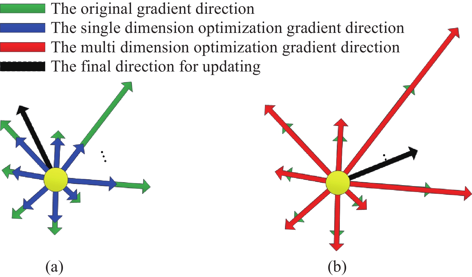
Figure 1. The different effects when using different optimization strategy.
3. A Novel Adaptive Learning Rate Algorithm
With the increasing of the dimension and complexity of the neural network, more and more saddle points have appeared in the objective functions. Hence, the gradient descent methods face more challenges. The optimization trajectory jumps out of the saddle point very slowly and guides the optimization process to the local minimum point following the small gradient value direction due to the facts that, many gradient values of the multi-dimension neural network are small, and some larger gradient values can be reduced by the current gradient optimization methods. This reduces the training speed.
Remark 1: In the neural network training, the optimization trajectory will be guided by the gradient direction. The AdaGrad-based optimization methods utilize the momentum parameter and the second-order-moment to revise the optimization direction (speed) and stability (accuracy). The optimization process will stop when the gradient vector is very small, even become zeros, which often happens at the saddle position or the optimal position. The optimization process hardly stops at the saddle position when the dimension of the neural network is huge, because it is difficult to make all the gradient components be zeros. In generally, the gradient descent method could guide the optimization trajectory move away from the saddle position easily.
For the optimization process, the gradient is significant to reduce the loss because it supplies a convinced optimization direction. When there exists a large gradient, we will prefer to select this direction to optimize the model (as shown in Figure 1(b)). Motivated by this idea, a novel adaptive learning rate optimization algorithm is proposed, which takes the relationship of all the gradient values into consideration. In order to quantize the multi-dimensional gradient contribution value, the function is used to produce the weight vector. The exponential decay rate parameter is imported to the algorithm to reduce the negative effects of the too fast decreasing learning rate. The detail of the multi dimension gradient optimization algorithm is shown in Algorithm 2, which is named as the M-AdaGrad algorithm and is based on the AdaGrad algorithm.
| Algorithm 2 M-AdaGrad algorithm |
| Require: Learning rate (Recommended default value: 0.001); |
| Require: Exponential decay rate parameter: (Recommended default value: 0.99); |
| Require: Exponential decay rate parameter: (Recommended default value: 1); |
| Require: A small constant value to make sure that the numeral computing stable (Recommended default value: 10−8); |
| Require: Initialed value of ; |
| 1: Initial the value of the second-order moment: ; |
| 2: Initial the time step, ; |
| 3: while Do not fit the stop condition do |
| 4: Sampling samples from the training data set as the mini batch data whose labels are ; |
| 5: Compute the gradient: ; |
| 6: Update the multi-gradient information parameters: , where , is the number of the parameters needed optimized; |
| 7: Revise the multi-gradient weight value parameters: , where ; |
| 8: Revise the exponential decay rate: , where ; |
| 9: Update the biased second-order moment estimation: (Application on each element); |
| 10: Update the computation: (Application on each element); |
| 11: Update the parameters: ; |
| 12: ; |
| 13: end while |
The main innovation in Algorithm 2 is the import of the multidimension gradient information. The function is utilized to describe the optimization ability in different gradient directions, and has the following good characteristics.
1) Saturation characteristic. When there are only a few gradient directions, the weight of these directions would not be very big because the maximum value of the function is 1. This guarantees the weight holds in a controlled range so that the ‘gradient explosion’ situation could be efficiently prevented as shown in Figure 2.
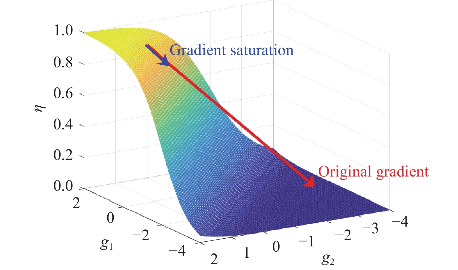
Figure 2. Gradient explosion restraining.
2) Significant preferences in directions of large gradients. The basic function of the is the exponential function , and the weight of the larger gradient direction will be further enhanced compared with the small gradient direction, which is shown in Figure 3. The exponential decay rate parameter is used to adjust the distribution of the weight vector.
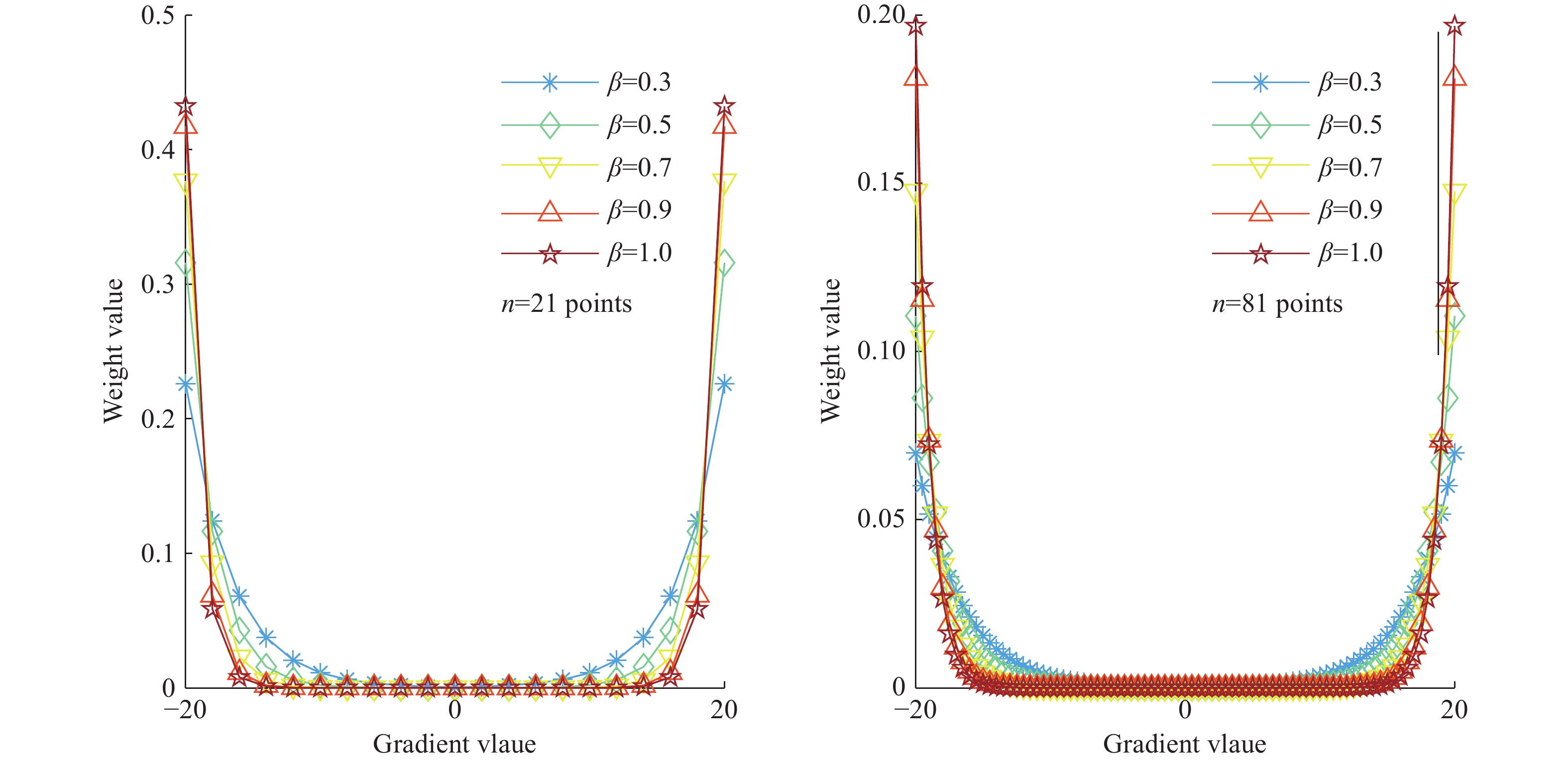
Figure 3. The weight vector distribution with different dimension and .
3) The uniform distribution when the inputs are small. The optimization trajectory usually changes slowly when going around the local minimum point, because all the gradient components are very small. In this case, the weight value will converge to , where is the number of the parameters to be optimized. Figure 4 shows the change of weights in the gradient range from − to for n=11, where the weight value vector is distributed almost uniformly. This indicates that the final direction of the optimization will be the same as the original gradient vector direction. Hence, the optimization process could reach local minimum solution stability. In other words, this method holds the advantage of the traditional gradient descent method when the search point is close to the optimal solution.
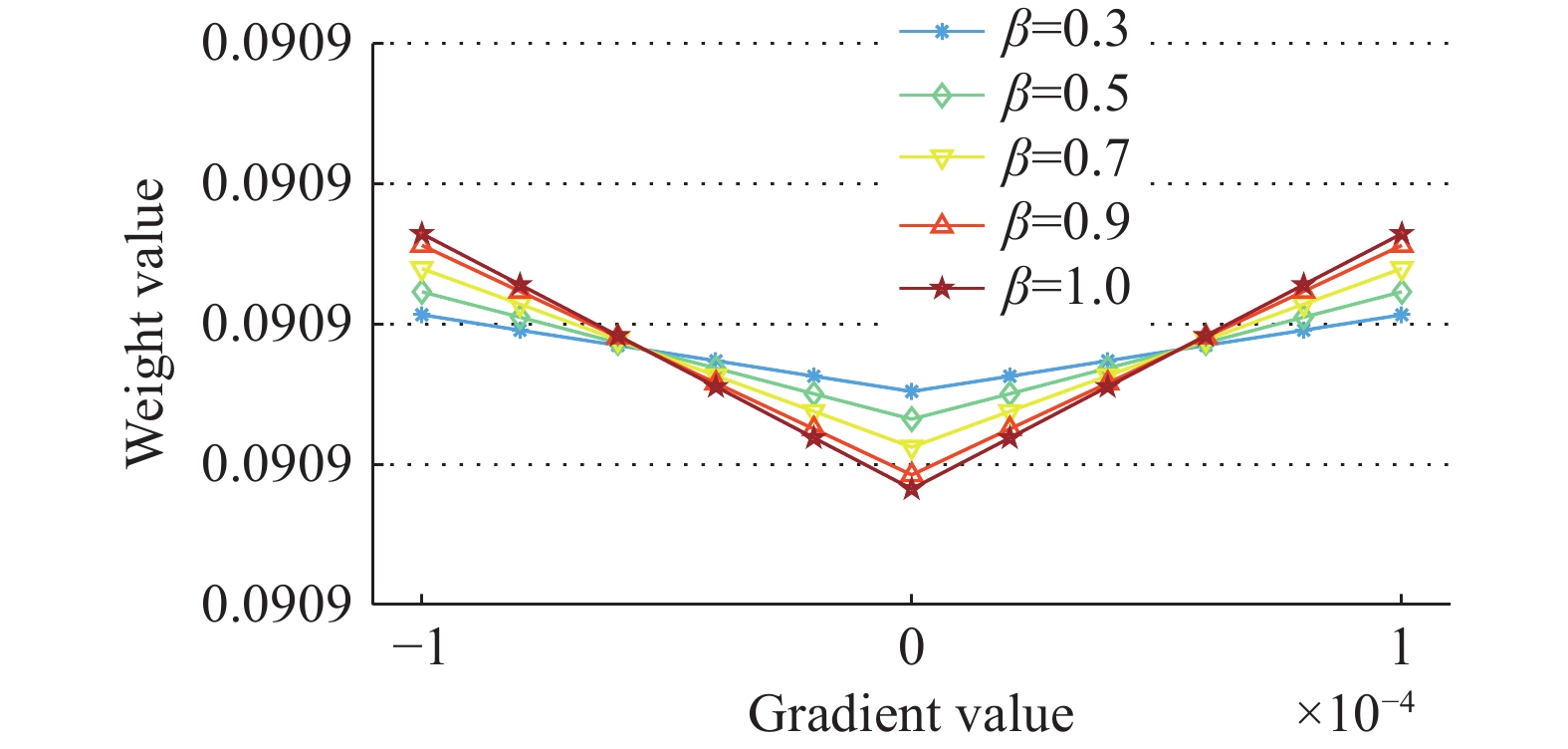
Figure 4. The weight value vector distributed almost uniformly.
Remark 2: It should be noted that the exponential decay rate parameter in is designed to balance the enhancement ratio of the multi-gradient direction. When the value of is larger (in the range of ), the ratio of the multi gradient direction would be enhanced more significantly, which can be seen in Figure 3. Meanwhile, this parameter could prevent the numerical computation error. Almost all computation platforms (e.g. MATLAB) have the limitation of the biggest computing numerical value. There might be overflow caused by the function when the input gradient value is big. The parameter can be set artificially to constrain the magnitude of the power of the exponential function, which provides a way to deal with this kind of problem. It is still recommended that preprocess the training data to make sure that the training process work well. This is good to improve the performance of the neural networks.
Furthermore, four parameters should be initialized including the learning rate , the exponential decay rate parameters and , and the small constant in the proposed M-AdaGrad algorithm. Especially, the exponential decay parameter is designed to adjust the exponential decay of the momentum estimate . When the modified function degenerates to , the form of the exponential decay of momentum estimation will be the same as the RMSProp. By introducing the modified , the learning rate will change adaptively according to the gradient value. For the large gradient direction, the learning rate attenuation will be small, so as not to weaken its guiding significance for the optimization process. Meanwhile, this exponential decay rate can also ensure a small learning rate when the optimization trajectory is close to the optimal solution. Hence, the optimization process can converge to the target point.
4. Simulation
To identify the advantages and characteristics of the proposed M-AdaGrad, a visible simulation experiment is carried out in this section. A multi-parameter nonconvex optimization task is designed using a set of sigmoid based functions given by (2).
where and are the parameters to be optimized, and , , , , and are constant parameters. Six sigmoid-based functions are imported to build a nonconvex optimization face and the corresponding parameters are presented in Table 1.
| Functions | ||||||
| 6 | 0.1 | −2 | 10 | 4 | 9 | |
| 4 | 0.1 | 7 | −10 | 20 | 4 | |
| 7 | 0.8 | 10 | 5 | 4 | 17 | |
| 7 | 0.8 | −12 | −5 | 14 | 25 | |
| 6 | 0.7 | −10 | 10 | 4 | 9 | |
| 10 | 1.3 | 1 | −1 | 25 | 40 |
The loss function is designed as follows based on the above function set.
where the training data set is presented in Table 2 and is the number of the training data. The parameters and are the targets to be optimized by minimizing the loss function .
| variable | 1 | 2 | 3 | 4 | 5 |
| x | 0.33 | 0.31 | 0.32 | 0.2 | 0.22 |
| y | 0.64 | 0.63 | 0.61 | 0.39 | 0.42 |
| variable | 6 | 7 | 8 | 9 | 10 |
| x | 0.02 | 0.17 | 0.06 | 0.2 | 0.6 |
| y | 0.02 | 0.19 | 0.06 | 0.22 | 0.151 |
Combining the data and the loss function mentioned above, a complex optimization space can be obtained which includes four different local minimum positions and two different local maximum positions as shown in Figure 5.
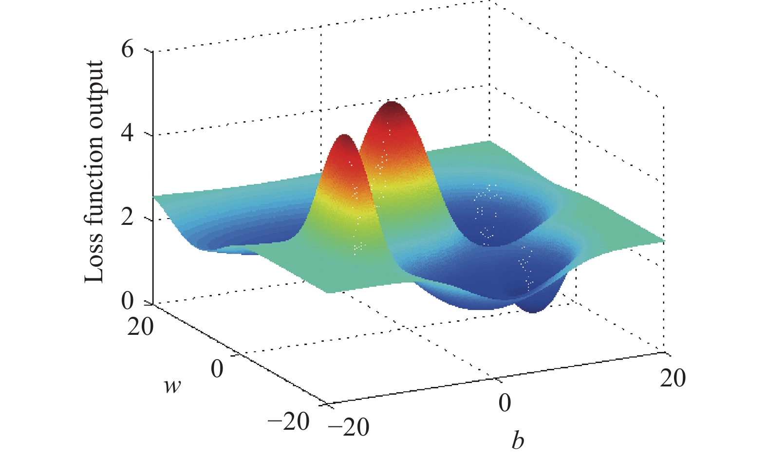
Figure 5. The 3D visible plane of the loss function.
In the deep learning training process, the optimization result will finally converge to a local minimum solution, and the initial points play important roles during this process. To fully verify the performance of the proposed M-AdaGrad in different situations, three experiments are designed at different initial points , and . In the first experiment, the starting point is between two local minimum positions; in the second experiment, there are three local minimum positions in front of the starting point; and in the third experiment, the starting point is close to a local minimum position. In every experiment, two optimization trajectories are presented using the proposed new algorithm and the general algorithm. The iteration number is set to be a constant value to compare the converging speed of the two optimization algorithms.
4.1. The First Experiment
The optimized trajectory result of the first experiment is shown in Figure 6. Although the optimization trajectories are opposite, both of them converge to a local minimum point, which shows the effectiveness of the proposed method. What is more, the trajectory of M-AdaGrad is more sparse near the initial position, and approaches the local optimal point more directly than the trajetory of the general optimization.
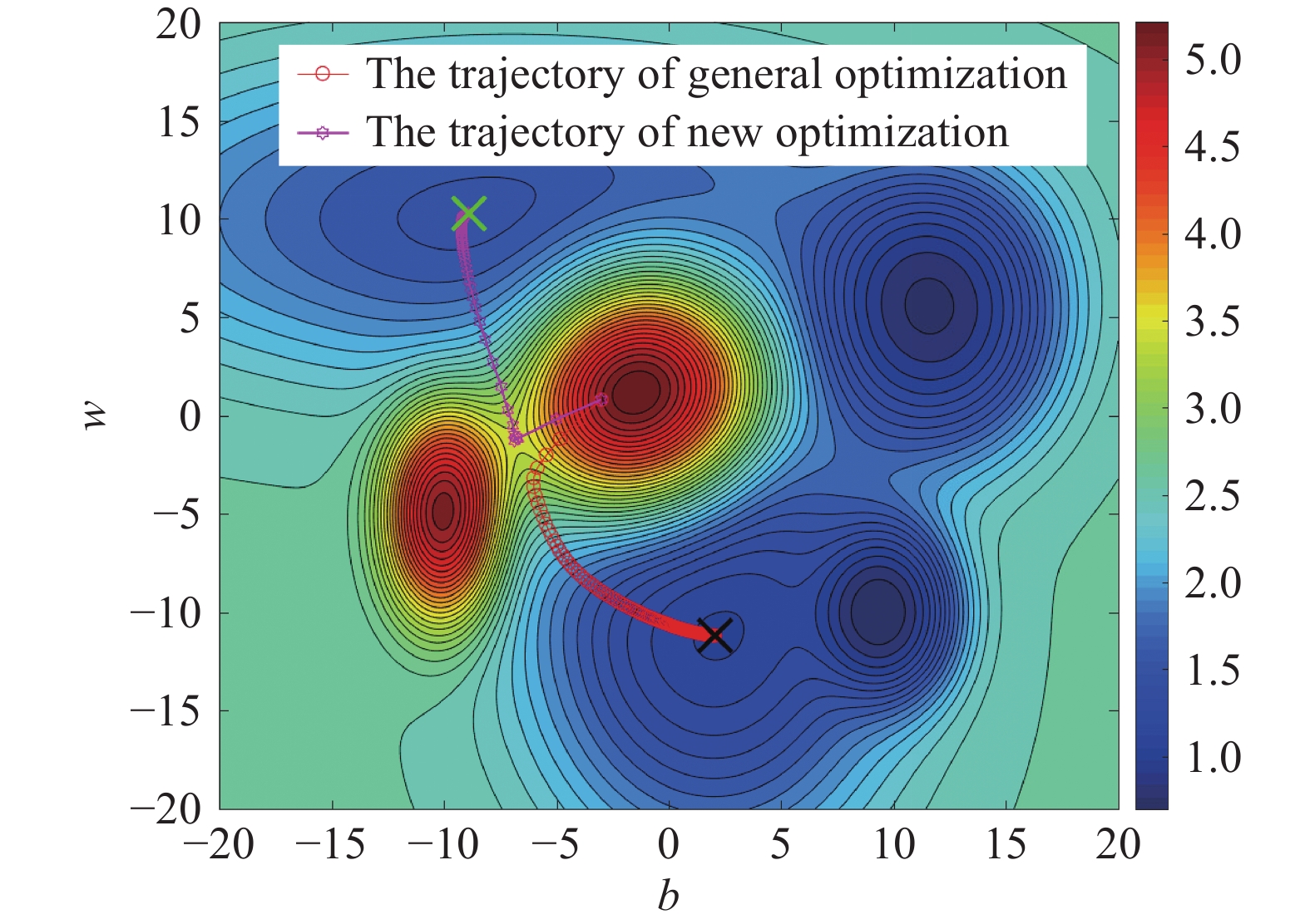
Figure 6. The optimized trajectory of the first experiment
Figure 7 shows the gradient curves of every direction/dimension. The gradients optimized by the proposed M-AdaGrad (both and ) converge to zeros much faster than the gradients in general optimization algorithms. Furthermore, combined with the weight curves in Figure 8, M-AdaGrad tends to assign more weights to the large gradient directions. Therefore, the gradient curves of M-AdaGrad fluctuate more heavily especially around the saddle point, which indicates that M-AdaGrad is also helpful to the optimization process in escaping the saddle point efficiently.
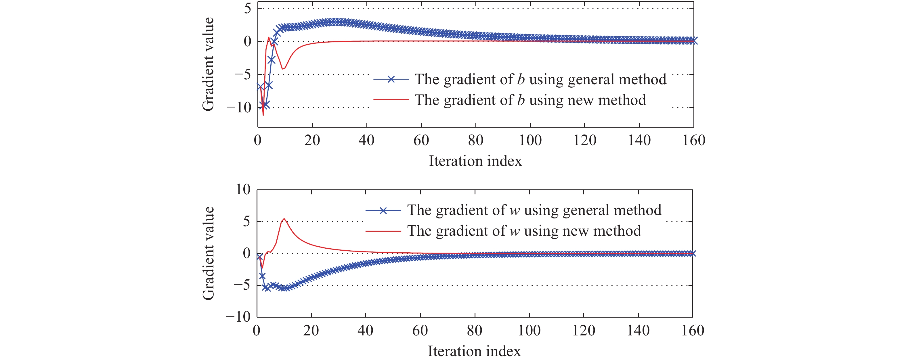
Figure 7. The gradient curves of every gradient direction of the first experiment.
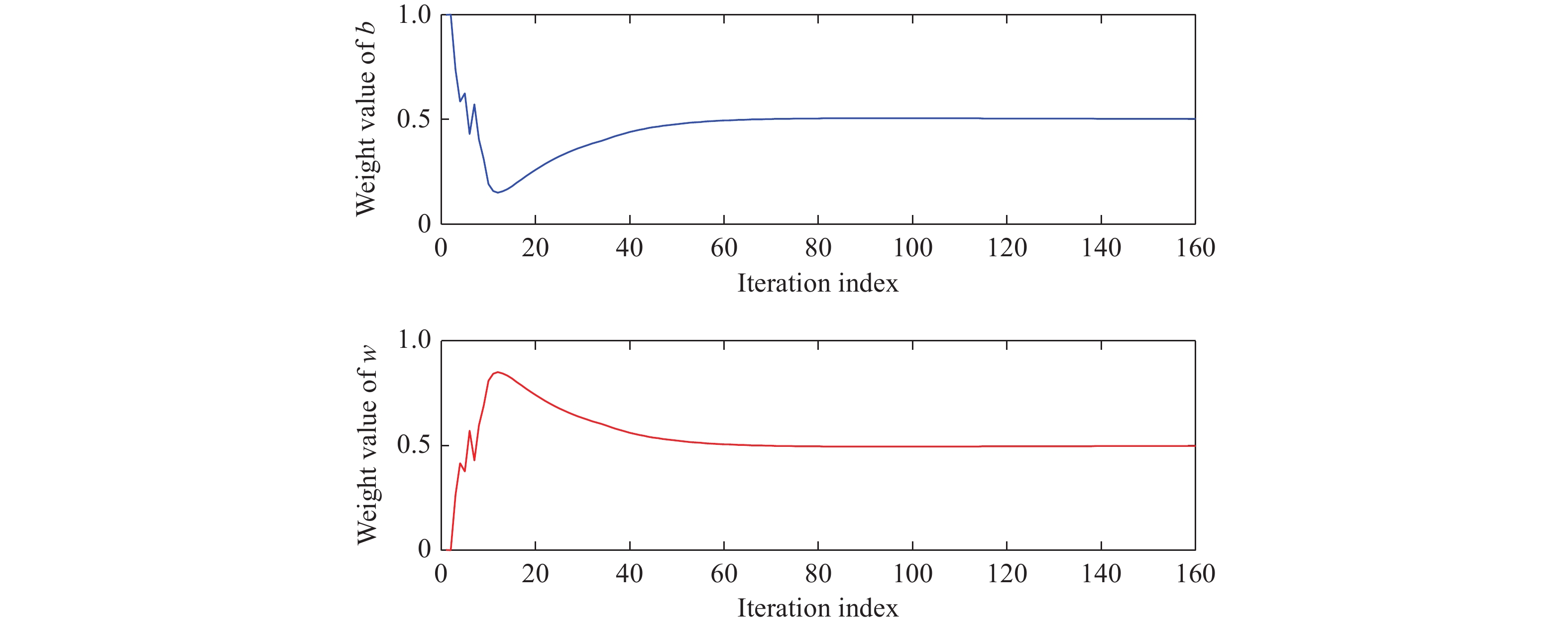
Figure 8. The weight vector of the learning rate of the first experiment.
Figure 8 also shows that the weight in M-AdaGrad converges to (this value will be when there are parameters), which indicates that the weight value will not influence the main direction when the optimization trajectory is close to the target point. This characteristic could be utilized to judge whether the optimization process converges or not, and design a corresponding stopping condition for training.
4.2. The Second Experiment
The second experiment simulates another situation where two local minimum positions exist in front of the initial point. Figure 9 presents the optimized trajectories of the two different gradient descent optimization algorithms. In general optimization algorithms, the learning rate is too much weakened in large gradient directions, which leads to the increased influence of small gradient directions on optimization, especially near the saddle point where the gradients of all parameters are relatively small and the small gradient directions even dominate the optimization route. This results in that the optimization trajectory bypasses a lower local minimum position (the red line in Figure 9). This drawback is improved by the M-AdaGrad algorithm, in which the weight is enhanced in the direction of large gradients. Hence, the optimization trajectory will approach a relatively smaller local minimum position, which means a better optimization result.
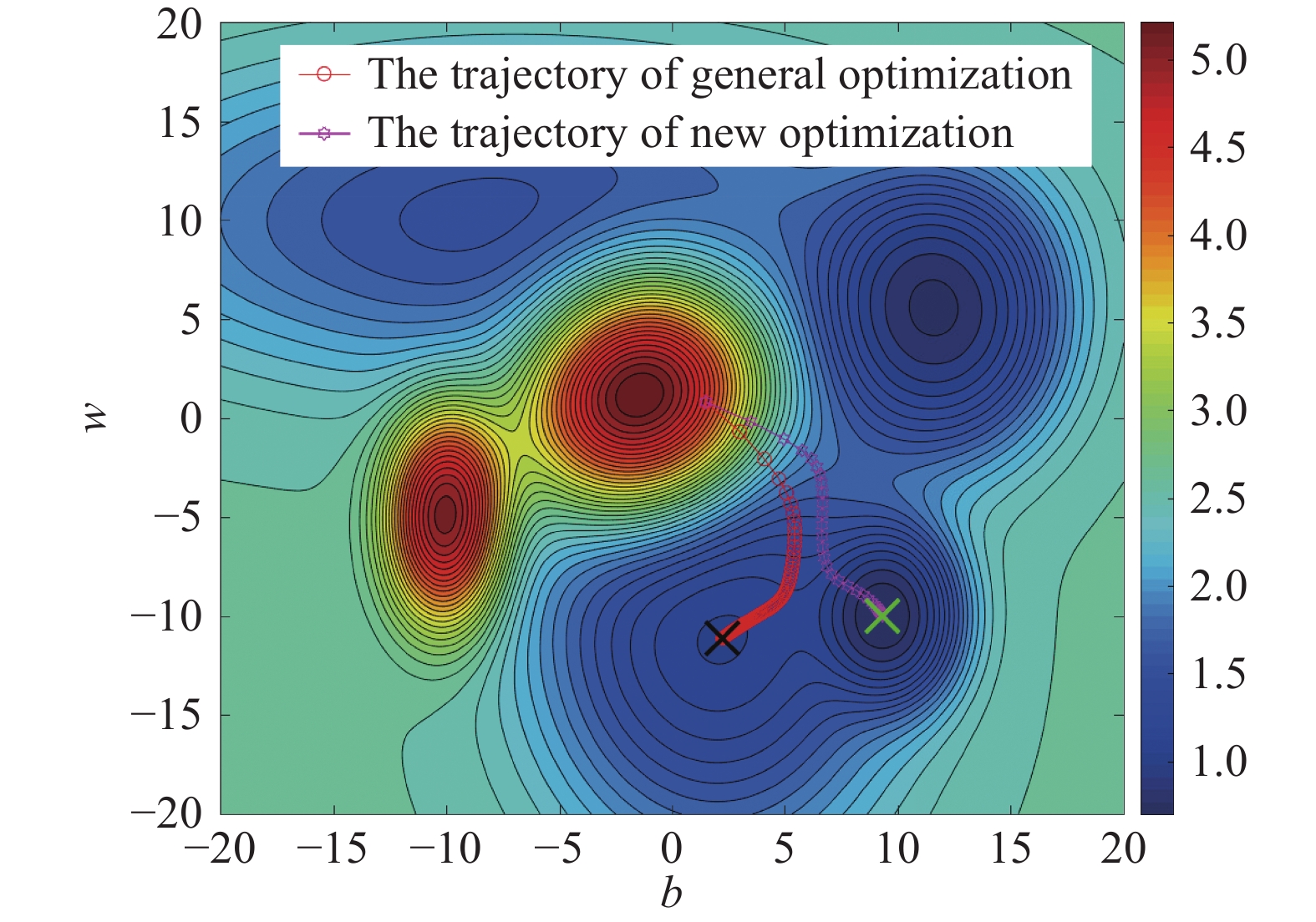
Figure 9. The optimized trajectory of the second experiment.
Figure 10 and Figure 11 show the gradient curves for the two parameters and the corresponding weight values. The gradient curves of the general algorithm in Figure 10 shows that the optimization speed is slow, even when the gradient is larger that that of the proposed algorithm, which again verifies that the information of the larger gradient directions is not fully used in the general algorithm. In addition, same as the first experiment, the weight in this experiment also converges to where .
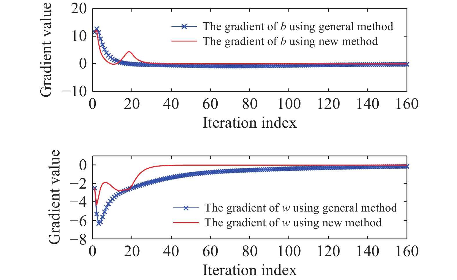
Figure 10. The gradient curves of every gradient direction of the second experiment.
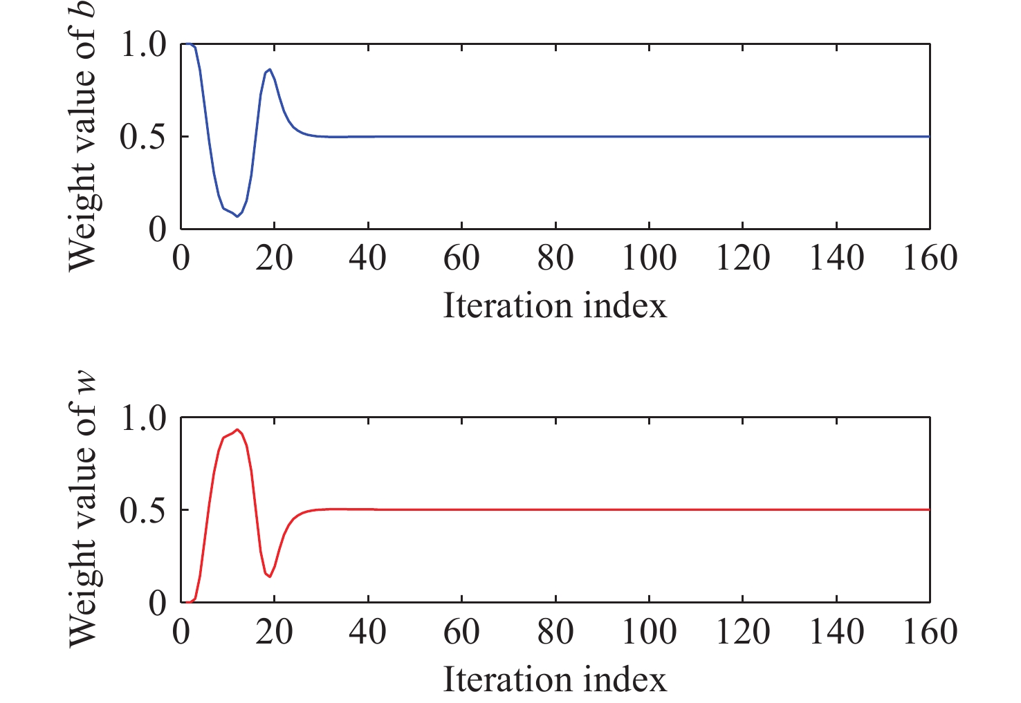
Figure 11. The weight vector of the learning rate of the second experiment.
4.3. The Third Experiment
The third experiment is carried out under the condition that there is only one local minimum point near the initial point. In this experiment, the general optimization algorithm and the proposed M-AdaGrad algorithm eventually converge around the same minimum point, but the optimization trajectories of the two algorithms are different. Figure 12 shows that M-AdaGrad can efficiently shorten the optimization trajectory and stably converge to the local minimum position. Furthermore, although the final optimization results are very close, the objective function value at the convergence point of M-AdaGrad is still slightly smaller than that of the general optimization algorithm. In addition, similar to Figure 8 and Figure 11, the weights in Figure 13 eventually converges to 1/2 as expected, which demonstrates that the M-AdaGrad algorithm is able to stably adjust the convergence weights.
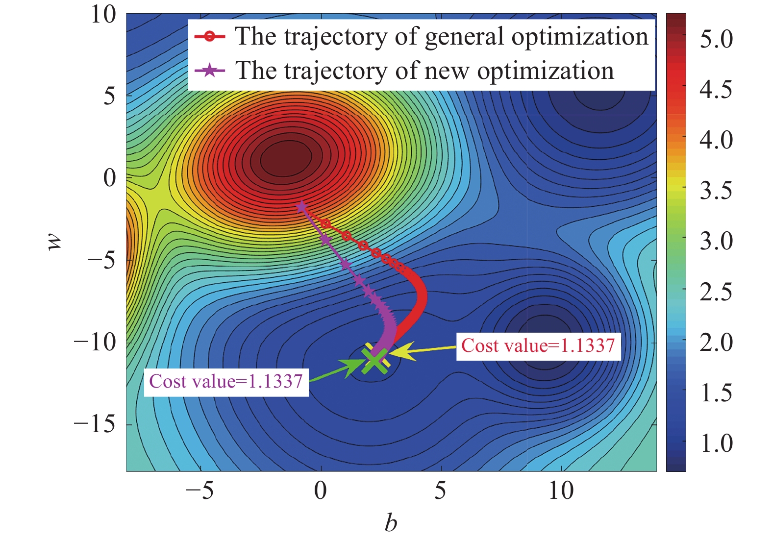
Figure 12. The optimized trajectory of the third experiment.
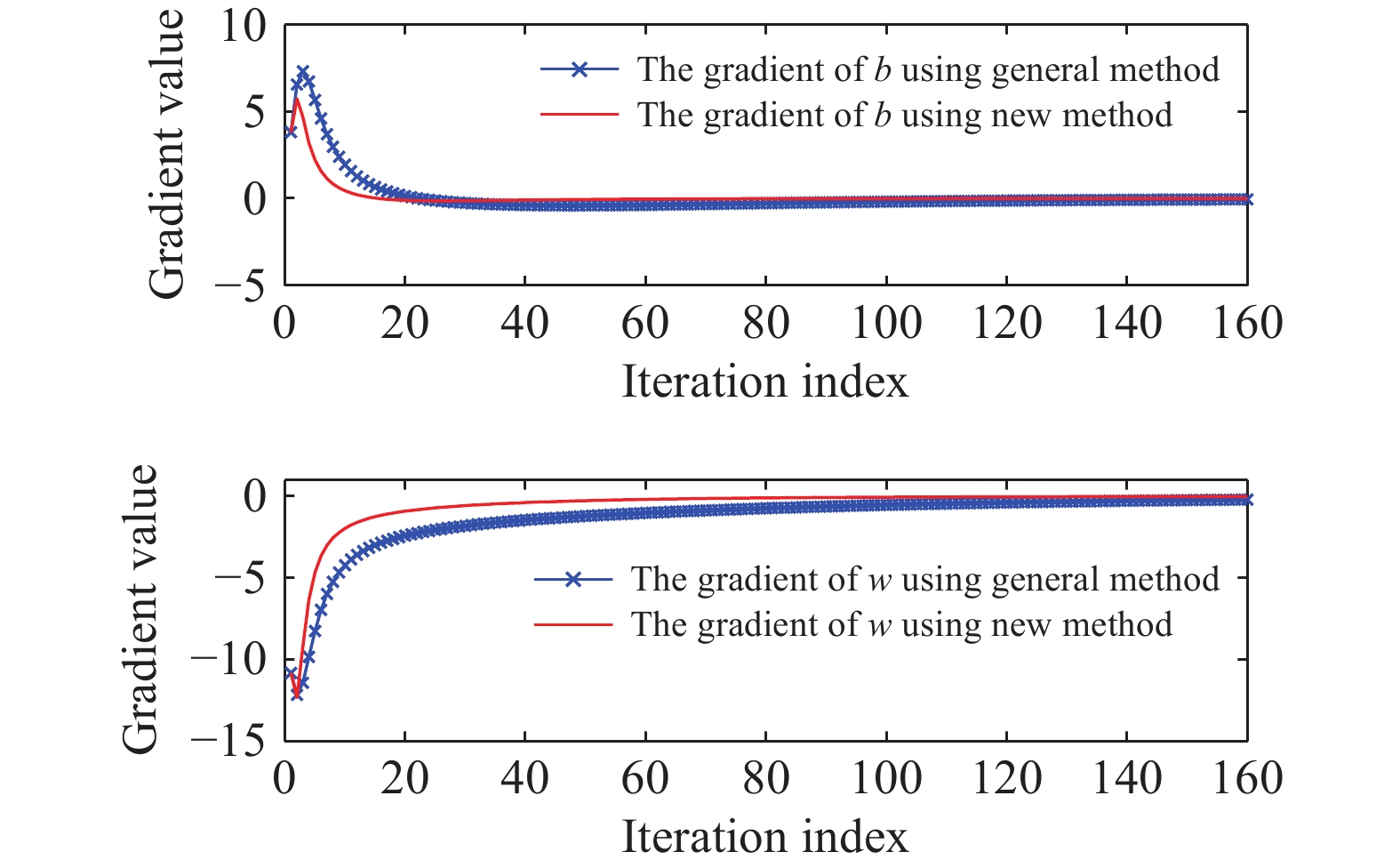
Figure 13. The gradient curves of every gradient direction of the third experiment.
5. Applications
To further verify the practical value of the proposed algorithm, we apply M-AdaGrad to network training to minimize the loss function and compare M-AdaGrad with other gradient descent optimization algorithms.
The mixed national institute of standards and technology database (MNIST) is a public computer vision dataset that contains 70000 grayscale images of handwritten numbers. Each image contains 784 (28 * 28) pixels, which can be transformed into a one-dimensional array of length 784 and used as input features. A fully connected neural network can be used for MNIST training to generate similar handwritten digital images. The loss function of this network can be written as (4).
where is the distribution that the detected images belong to, is the generator network, is the output of the generator network, is the distribution that the target images belong to, and is the discriminator network. The activation function of the hidden layers is the rectified linear unit (ReLU) and the activation function of the output layers (including the generator network and discriminator network) is the sigmoid function.
We use the Adam algorithm and M-AdaGrad to optimize the loss function, respectively, with the same training parameters. Figure 14 shows the comparison of the training results of the generated network after a fixed number of iterations by M-AdaGrad and Adam. Figure 14 shows that, although the network trained by M-AdaGrad still contains some noises, it is able to generate a relatively legible handwritten digital image after 1200 iterations. In contrast, the shape of the numbers is hard to be recognized in the images generated by the Adam trained network. Previous experiments on the sigmoid-based functions show that M-AdaGrad can minimize the objective function to a more optimal value with a faster speed than Adam. This is also verified in the application to network training based on the public dataset (i.e. the MNIST dataset).
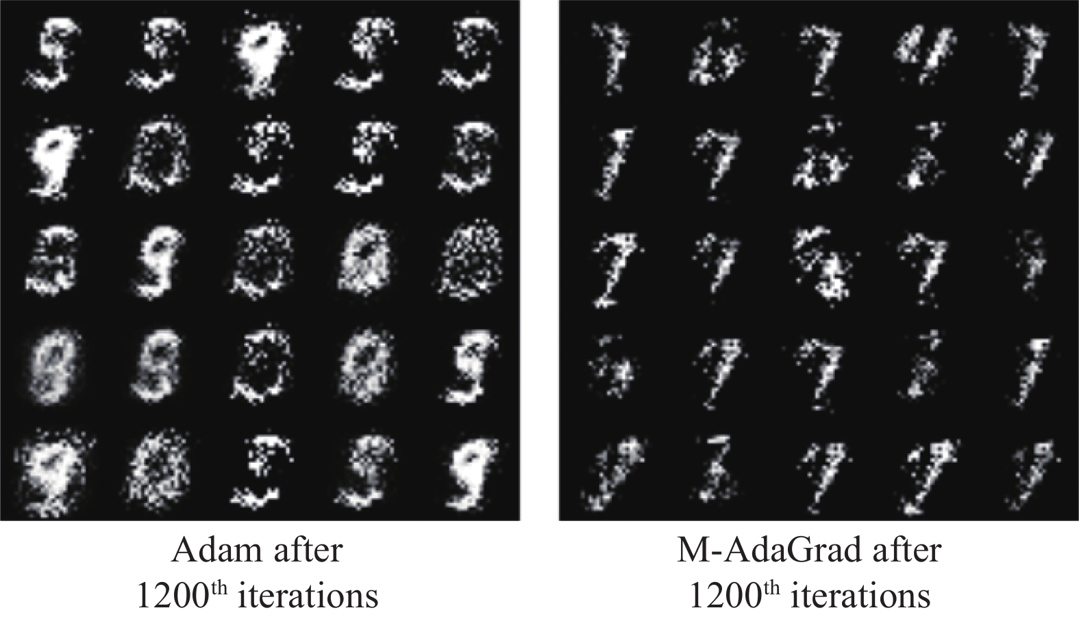
Figure 14. Comparison between two different optimization methods on the public dataset.
As neural networks are extensively applied to finish practical industrial tasks, we next apply M-AdaGrad to a specific industrial case. Crack detection is one of the important tasks in visual NDT, which is widely used to maintain large equipment in the industrial process [30, 31]. In visual NDT, the cracks in the detection image cannot be accurately characterized compared with the tangible object identification such as face detection. Deep learning is a good way to build a model to process the visual NDT images and has been widely used in recent years. In this case, an efficient optimization algorithm is required to train the model more fast and accurate.
The magnetic optical image (MOI) is one of the visual NDTs. To identify the crack from the detected image which is shown in Figure 15, the GAN method is used to segment and enhance the image. The SGD, Adam and proposed M-AgaGrad are used to train the network, respectively, and the loss function is shown as follows:
where is a hyperparameter, is the Frobenius norm whose definition is , is the generator network, is the detected image, is the target image, and is the general loss function shown in (4).
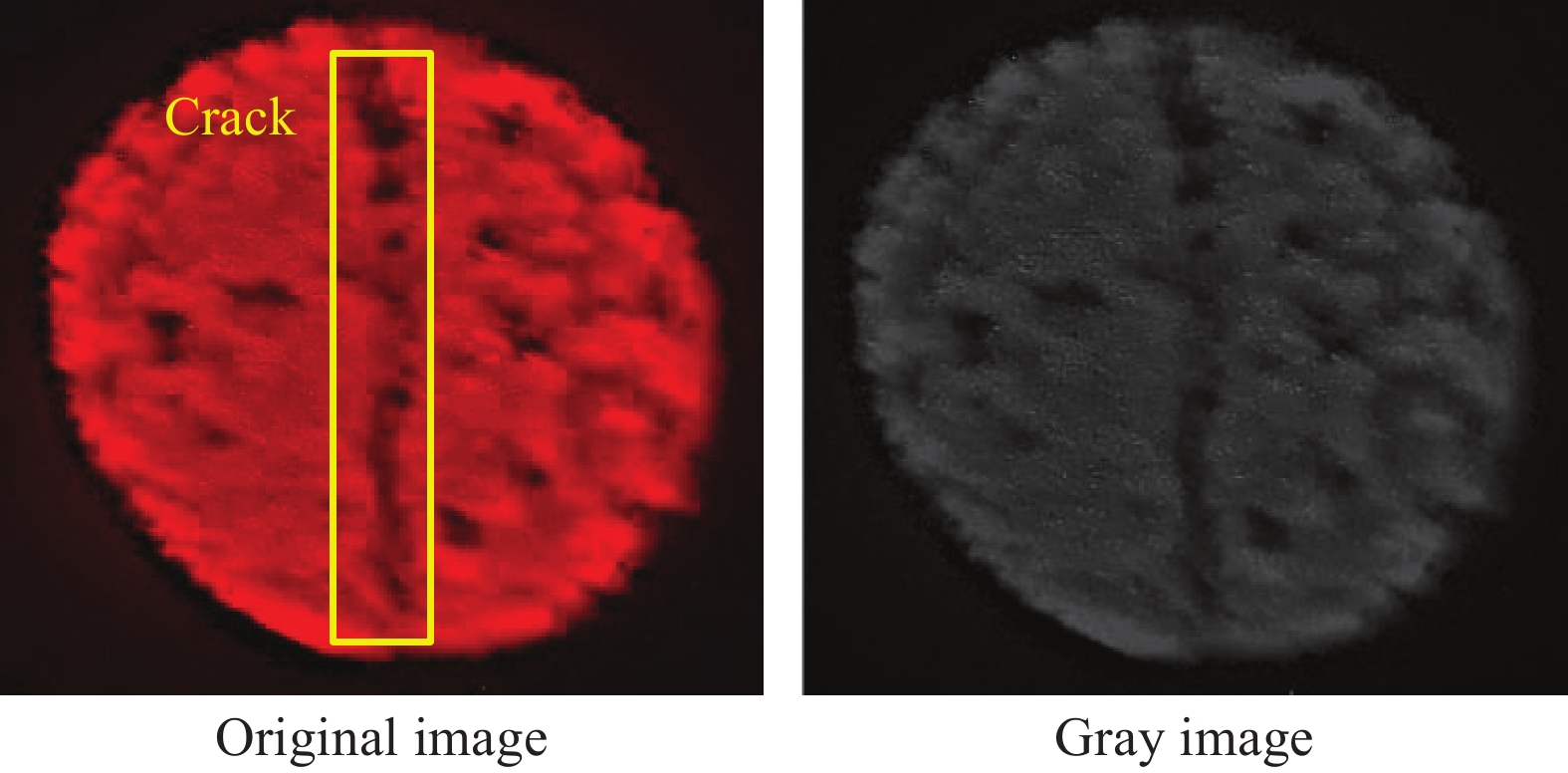
Figure 15. The detected MOI image and its gray image.
In the loss function, the performance function is used to stop the training process, which shows the error between the reconstructive image and target image. The initialization parameters of the GAN are the same for each optimization algorithm.
Remark 3:
The target image (ground truth) in the neural network is obtained according to the known features (shape and size) of the crack. The target image is full of experiential knowledge and is only used as a part of the training set. When a trained neural network is used for actual detection, the shape of the defect is unknown.
Figures 16-18 show the error curves of different optimization algorithms under the three cases mentioned in Section. 4. In Figure 16, compared with the SGD, the error curves of the two adaptive learning rate algorithms (Adam and M-AdaGrad) both decline as the iteration number increases. The error curve of Adam decreases rapidly at the beginning, and converges to a larger local minimum point with large fluctuations. In contrast, the error curve of the M-AdaGrad algorithm converges to a smaller error with a better local optimal point.
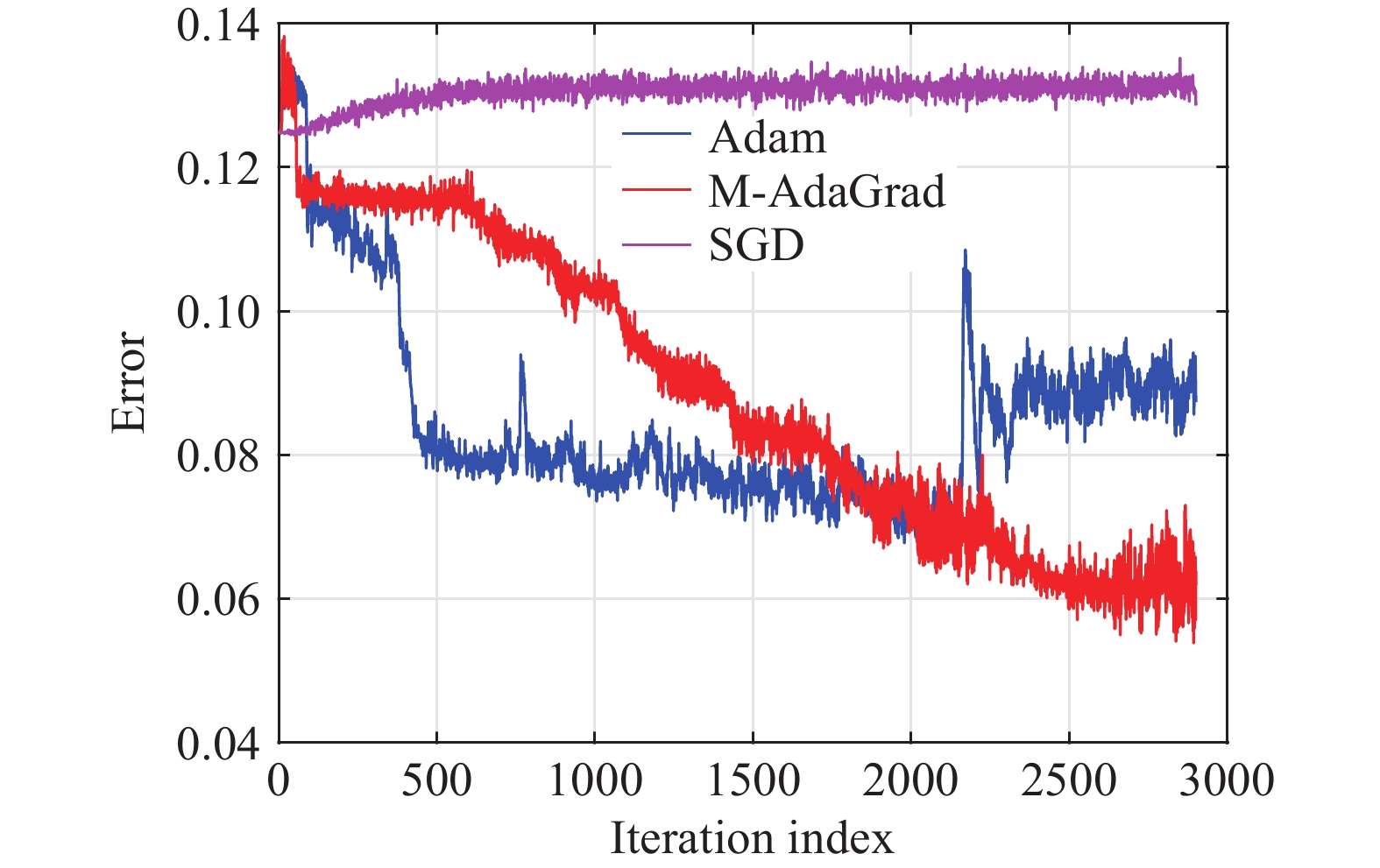
Figure 16. The error using different optimizations under the case of the first experiment.
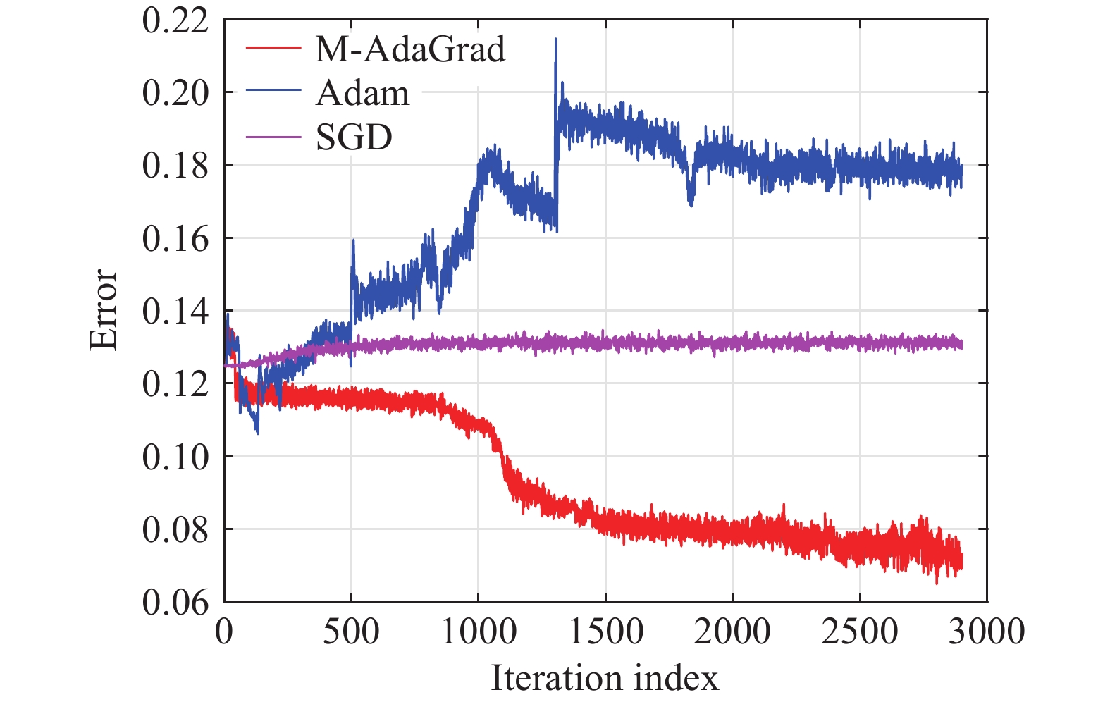
Figure 17. The error using different optimizations under the case of the second experiment.
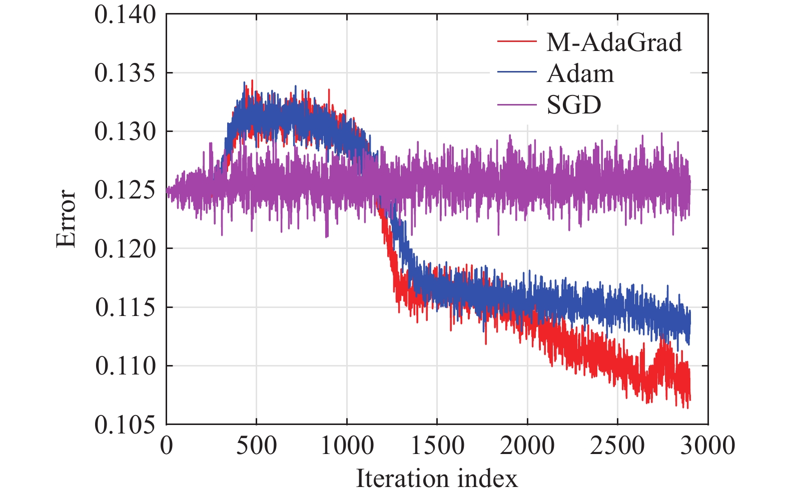
Figure 18. The error using different optimizations under the case of the third experiment three.
In Figure 17, the three error curves change towards different directions. The error curve of the SGD algorithm is approximately maintained at the initial position, indicating that the initial value is near the saddle point and it is hard for the SGD to make the optimization process jump out of the saddle point. The Adam algorithm can jump out of the saddle point quickly, but the error gradually increases and finally converges to a position with greater errors. M-AdaGrad improves the disadvantage of Adam by jumping out of the saddle point quickly, iterating the optimization process along the direction of the error reduction, and finally converging to a position where the error is smaller than the initial value.
Figure 18 shows the error curves under the last case in Section. 4. The Adam and M-AdaGrad algorithms converge around the same local minimum point, hence the error curves are almost the same. The main difference is that the M-AdaGrad algorithm is faster than the Adam algorithm in reaching the direction along which the error decreases. In addition, the convergence solution of M-AdaGrad is smaller than that of Adam in a limited iteration time.
M-AdaGrad also has its limitations. Figures 16-18 show that M-AdaGrad can quickly reduce the objective function/loss function to a relatively small value, but the negative impact is that there may be a relatively gentle decline rate that maintains for a period. This indicates that M-AdaGrad may have a decrease in model sensitivity with the increase of model sensitivity. Nevertheless, the experiments also show that M-AdaGrad can still converge to a lower value than Adam and SGD, if the iteration number increases. The guiding significance of this limitation is that M-AdaGrad has a clear advantage, if we want to get a pre-trained result quickly in a short time. If we want to get a more accurate training result, we need to increase the iteration number. It is worth noting that even if we increase the iteration number, the performance of M-AdaGrad is still better than Adam and SGD in terms of the accuracy and convergence speed.
Figure 19 is the reconstructive image which is generated by the GAN optimized using the proposed algorithm, and the image is enhanced and segmented well for the crack identification. The experiment in this specific industrial case shows that the proposed M-AdaGrad is a novel gradient descent optimization algorithm which can ensure good training effects of neural networks, while improving the training efficiency.
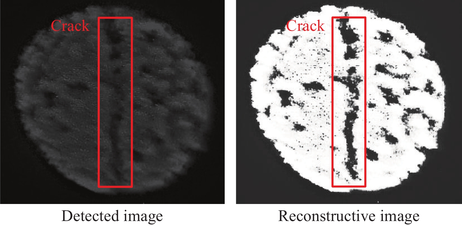
Figure 19. The reconstructive image using GAN.
6. Conclusion
In this paper, a novel multi-dimension SGD-based adaptive learning rate optimization algorithm (M-AdaGrad) has been proposed, which fuses the gradients of all parameters and produces weight vectors based on the softmax function to adaptively adjust the learning rate. The simulation experiments under three different initial points have verified that the optimized trajectory of the proposed algorithm is more influenced by the large (other than small) gradient components. This helps improve the training speed and guide the loss function to a smaller local optimal solution to improve the training effect of the network. In an industrial case (the magneto-optical NDT), it has been shown that compared with the widely used SGD and Adam algorithms, M-AdaGrad has superior performances in jumping out of the saddle point faster and converging to an optimal position with lower errors. To sum up, M-AdaGrad shows great potentials for industrial applications. In the future, we will apply M-AdaGrad to more application scenarios to fully explore its potential.
Author Contributions: Yiping Liang: investigation, data curation, writing-original draft, writing-review & editing; Lulu Tian: conceptualization, methodology, supervision, writing-original draft, writing-review & editing; Xu Zhang: formal analysis, supervision; Xiao Zhang: formal analysis, supervision; Libing Bai: supervision, funding acquisition, project administration. All authors have read and agreed to the published version of the manuscript.
Funding: This work was supported in part by the National Natural Science Foundation of China under Grant U2030205 and Sichuan Science and Technology Planning Project 2022JDJQ0040.
Data Availability Statement: Not applicable.
Conflicts of Interest: The authors declare no conflicts of interest.

References
- Yu, N.X.; Yang, R.; Huang, M.J. Deep common spatial pattern based motor imagery classification with improved objective function. Int. J. Network Dyn. Intell., 2022, 1: 73−84. doi: 10.53941/ijndi0101007
- Zeng, N.Y.; Wu, P.S.; Wang, Z.D.; et al. A small-sized object detection oriented multi-scale feature fusion approach with application to defect detection. IEEE Trans. Instrum. Meas., 2022, 71: 3507014. doi: 10.1109/TIM.2022.3153997
- Perdios, D.; Vonlanthen, M.; Martinez, F.; et al. CNN-based image reconstruction method for ultrafast ultrasound imaging. IEEE Trans. Ultrason. Ferroelectr. Freq. Control, 2022, 69: 1154−1168. doi: 10.1109/TUFFC.2021.3131383
- Li, H.; Wang, P.; Shen, C.H. Toward end-to-end car license plate detection and recognition with deep neural networks. IEEE Trans. Intell. Transport. Syst., 2019, 20: 1126−1136. doi: 10.1109/TITS.2018.2847291
- Abdelhamid, A.A.; El-Kenawy, E.S.M.; Alotaibi, B.; et al. Robust speech emotion recognition using CNN+LSTM based on stochastic fractal search optimization algorithm. IEEE Access, 2022, 10: 49265−49284. doi: 10.1109/ACCESS.2022.3172954
- Lu, Y.J.; Tian, H.; Cheng, J.; et al. Decoding lip language using triboelectric sensors with deep learning. Nat. Commun., 2022, 13: 1401. doi: 10.1038/s41467-022-29083-0
- De Lope, J.; Graña, M. An ongoing review of speech emotion recognition. Neurocomputing, 2023, 528: 1−11. doi: 10.1016/j.neucom.2023.01.002
- Cai, L.N.; Cao, K.T.; Wu, Y.P.; et al. Spectrum sensing based on spectrogram-aware CNN for cognitive radio network. IEEE Wirel. Commun. Lett., 2022, 11: 2135−2139. doi: 10.1109/LWC.2022.3194735
- Minakova, S.; Stefanov, T. Memory-throughput trade-off for CNN-based applications at the edge. ACM Trans. Des. Autom. Electron. Syst., 2023, 28: 2. doi: 10.1145/3527457
- Zhang, X.Y.; Zhou, X.Y.; Lin, M.X.;
et al . ShuffleNet: An extremely efficient convolutional neural network for mobile devices. InProceedings of the IEEE Conference on Computer Vision and Pattern Recognition, Salt Lake City, UT, USA, 18–23 June 2018 ; IEEE: New York, 2018; pp. 6848–6856. doi: 10.1109/CVPR.2018.00716 - Tian, L.L.; Wang, Z.D.; Liu, W.B.; et al. A new GAN-based approach to data augmentation and image segmentation for crack detection in thermal imaging tests. Cogn. Comput., 2021, 13: 1263−1273. doi: 10.1007/s12559-021-09922-w
- Liu, K.H.; Ye, Z.H.; Guo, H.Y.; et al. FISS GAN: A generative adversarial network for foggy image semantic segmentation. IEEE/CAA J. Autom. Sin., 2021, 8: 1428−1439. doi: 10.1109/JAS.2021.1004057
- Li, Y.F.; Peng, X.Y.; Zhang, J.; et al. DCT-GAN: Dilated convolutional transformer-based GAN for time series anomaly detection. IEEE Trans. Knowl. Data Eng., 2023, 35: 3632−3644. doi: 10.1109/TKDE.2021.3130234
- Kordi Ghasrodashti, E.; Sharma, N. Hyperspectral image classification using an extended auto-encoder method. Signal Process. Image Commun., 2021, 92: 116111. doi: 10.1016/j.image.2020.116111
- Cao, X.; Luo, Y.H.; Zhu, X.Y.; et al. DAEANet: Dual auto-encoder attention network for depth map super-resolution. Neurocomputing, 2021, 454: 350−360. doi: 10.1016/j.neucom.2021.04.096
- Wang, Y.S.; Yao, H.X.; Zhao, S.C. Auto-encoder based dimensionality reduction. Neurocomputing, 2016, 184: 232−242. doi: 10.1016/j.neucom.2015.08.104
- Frame, J.M.; Kratzert, F.; Raney II, A.; et al. Post-processing the national water model with long short-term memory networks for streamflow predictions and model diagnostics. J. Am. Water Resour. Assoc., 2021, 57: 885−905. doi: 10.1111/1752-1688.12964
- Zhang, Y.Z.; Xiong, R.; He, H.W.; et al. Long short-term memory recurrent neural network for remaining useful life prediction of lithium-ion batteries. IEEE Trans. Veh. Technol., 2018, 67: 5695−5705. doi: 10.1109/TVT.2018.2805189
- Lino, M.; Fotiadis, S.; Bharath, A.A.; et al. Multi-scale rotation-equivariant graph neural networks for unsteady Eulerian fluid dynamics. Phys. Fluids, 2022, 34: 087110. doi: 10.1063/5.0097679
- Sabir, Z.; Raja, M.A.; Baleanu, D.; et al. Investigations of non-linear induction motor model using the Gudermannian neural networks. Therm. Sci., 2022, 26: 3399−3412. doi: 10.2298/TSCI210508261S
- Zhang, M.H.; Chen, Y.X. Link prediction based on graph neural networks. In
Proceedings of the 32nd International Conference on Neural Information Processing Systems, Montreal, Canada, 3–8 December 2018 ; Curran Associates Inc: Red Hook, 2008; pp. 5171–5181. - Liu, W.B.; Wang, Z.D.; Yuan, Y.; et al. A novel sigmoid-function-based adaptive weighted particle swarm optimizer. IEEE Trans. Cybern., 2021, 51: 1085−1093. doi: 10.1109/TCYB.2019.2925015
- Li, Y.Z.; Yuan, Y. Convergence analysis of two-layer neural networks with ReLU activation. In
Proceedings of the 31st International Conference on Neural Information Processing Systems, Long Beach, CA, USA, 4–9 December 2017 ; Curran Associates Inc: Red Hook, 2017; pp. 597–607. - Luo, X.; Liu, Z.G; Li, S.; et al. A fast non-negative latent factor model based on generalized momentum method. IEEE Trans. Syst. Man Cybern. Syst., 2021, 51: 610−620. doi: 10.1109/TSMC.2018.2875452
- Duchi, J.; Hazan, E.; Singer, Y. Adaptive subgradient methods for online learning and stochastic optimization. J. Mach. Learn. Res., 2011, 12: 2121−2159.
- Cao, Y.Z.; Das, S.; Van Wyk, H.W. Adaptive stochastic gradient descent for optimal control of parabolic equations with random parameters. Numer. Methods Partial, 2022, 38: 2104−2122. doi: 10.1002/num.22869
- Kingma, D.P.; Ba, J. Adam: A method for stochastic optimization. In
Proceedings of the 3rd International Conference on Learning Representations, San Diego, CA, USA, 7 –9 May 2015 ; ICLR, 2015; pp. 1–13. doi: 10.48550/arXiv.1412.6980 - Chen, J.R.; Jin, S.; Lyu, L.Y. A consensus-based global optimization method with adaptive momentum estimation. Commun. Comput. Phys., 2022, 31: 1296−1316. doi: 10.4208/cicp.OA-2021-0144
- Tieleman, T.; Hinton, G. Lecture 6.5-rmsprop: Divide the gradient by a running average of its recent magnitude. COURSERA: Neural Networks Mach. Learn., 2012, 4: 26−31.
- Tian, L.L.; Cheng, Y.H.; Yin, C.; et al. Design of the MOI method based on the artificial neural network for crack detection. Neurocomputing, 2017, 226: 80−89. doi: 10.1016/j.neucom.2016.11.032
- Bai, L.B.; Liang, Y.P.; Shao, J.L.; et al. Moran’s index-based tensor decomposition for eddy current pulsed thermography sequence processing. IEEE Trans. Instrum. Meas., 2021, 70: 6009212. doi: 10.1109/TIM.2021.3096277


